The workflow of classification is very similar to regression. Suppose we had some labelled data of different cartoon images; Tom and Jerry. The model will then identify which images are Jerry and which ones are Tom.
The difference between classification and regression
First, we would clean the data and then perform some exploratory data analysis on the data. We would also need to train the model to recognise Tom and Jerry. Then we would implement the algorithm with one of the different classifiers available and then we would evaluate the performance of the model.
Multi-class classification is a type of machine learning classification where the model is trained to classify instances into one of more than two classes. This differs from binary classification, where the model only distinguishes between two classes.
In multi-class classification, the algorithm needs to be able to identify and assign an input to one of the multiple categories. A common example is image recognition, where an algorithm categorises images into different categories like cars, animals, plants, etc.
Below is an example of the MNIST (Modified National Institute of Standards and Technology) dataset - this is a very popular dataset which is often found in scientific papers. It was first implemented in 1980 at a post office in the United States, in order for an algorithm to recognise handwritten post codes on envelopes, in order for the post code to be digitalised.
## Clean/Investigate the data
For this notebook we will be using the tips dataset from seaborn, which contains information about meals in a restaurant.
The “tips” dataset includes the following variables:
tip: The tip amount in dollars.
sex: The gender of the person paying the bill.
smoker: Whether the party had smokers or not.
day: The day of the week.
time: The time of day, for example, Dinner or Lunch.
size: The size of the party.
tips = sns.load_dataset('tips')tips.head()
   total_bill   tip     sex smoker  day    time  size
0       16.99  1.01  Female     No  Sun  Dinner     2
1       10.34  1.66    Male     No  Sun  Dinner     3
2       21.01  3.50    Male     No  Sun  Dinner     3
3       23.68  3.31    Male     No  Sun  Dinner     2
4       24.59  3.61  Female     No  Sun  Dinner     4
For this notebook the target variable will be smoker - whether the party had smokers or not. We will see how our model will manage to predict who is a smoker and who is not a smoker based on the data.
First we will identify the number of smokers and non-smokers we have in the dataset.
# number of smokers and non smokerstips['smoker'].value_counts()
smoker
No     151
Yes     93
Name: count, dtype: int64
One issue that we have straight away is that we have more No than Yes. This means it will be easier for the model to predict that someone isn’t a smoker as it will have more experience with No than it does with Yes. (more data with No). So we will keep this in mind when it comes to setting up our model as we may need to balance the classes.
# information about the dataset - are there any missing values?tips.info()
Return the features training set, the features test set, target train set, target test set.
X_train, X_test, y_train, y_test = train_test_split(X, y, test_size=0.2, random_state =2024)
5.3.3 Model Creation
In linear regression, we first set up an instance of the model that contained the algorithm we need but didn’t contain the data (yet). We then fit the model to the data. We will follow the exact same process for the decision tree classifier.
# set up instance of modelclf = DecisionTreeClassifier()# fit the model to the dataclf.fit(X_train, y_train)
DecisionTreeClassifier()
In a Jupyter environment, please rerun this cell to show the HTML representation or trust the notebook. On GitHub, the HTML representation is unable to render, please try loading this page with nbviewer.org.
DecisionTreeClassifier()
We can visualise this by using the below code. It converts the feature names from X into a list, and plots the decision tree with nodes colored based on class majority. The tree uses “No” and “Yes” to label its classes and displays the feature names at each decision node.
We can now evaluate the mode, using the same methods as we did for linear regression. First, we will create a variable called y_pred and run the X_test data on the model to get a series of predicted values.
# add y_pred and y_test to a df to comparedf_test_predict = pd.DataFrame({'y_test': y_test, 'y_predict' : y_pred})df_test_predict.head()
    y_test y_predict
239     No        No
238     No        No
170    Yes        No
156     No        No
134     No       Yes
From this small snippet of the dataframe, we can see that most values are predicted correctly (although not all).
We have some more metrics called the accuracy score, F1 score, recall score and precision score. These will help us evaluate the accuracy of our model.
# predicting on the training datay_train_estimated = clf.predict(X_train)
5.3.4.1 Accuracy score
# accuracy score of test dataaccuracy_score(y_test, y_pred)
0.5714285714285714
# accuracy score of training dataaccuracy_score(y_train, y_train_estimated)
0.9948717948717949
What do these two scores tell us about the model?
5.3.4.2 Precision score
For the precision score, we need to add a parameter called pos_label which will be set at Yes.
precision_score(y_test, y_pred, pos_label ='Yes')
0.3684210526315789
5.3.4.3 Recall score
recall_score(y_test, y_pred, pos_label ='Yes')
0.4375
5.3.4.4 F1 score
f1_score(y_test, y_pred, pos_label ='Yes')
0.4
5.3.4.5 Confusion Matrix
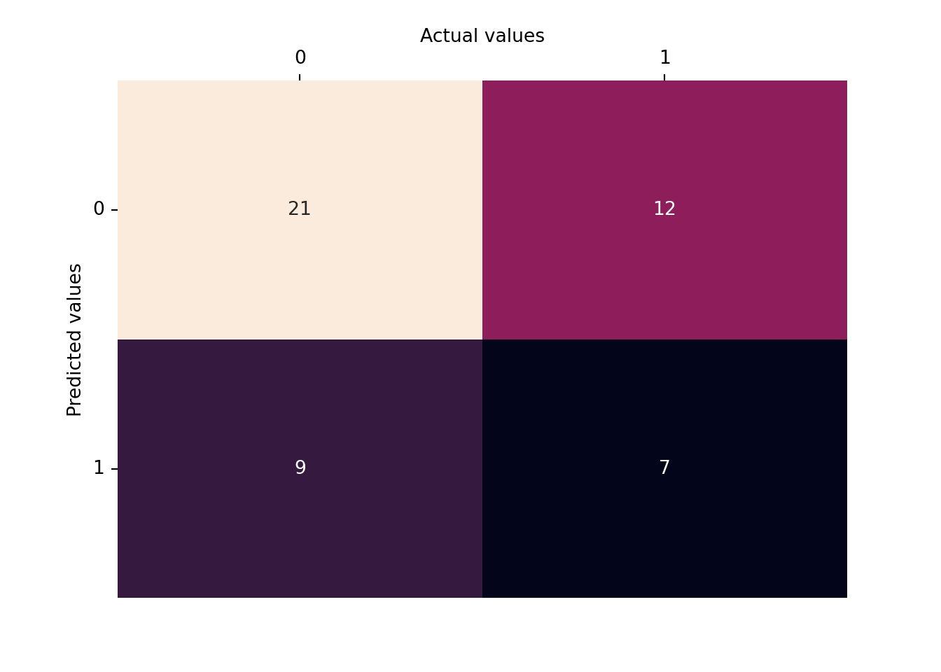
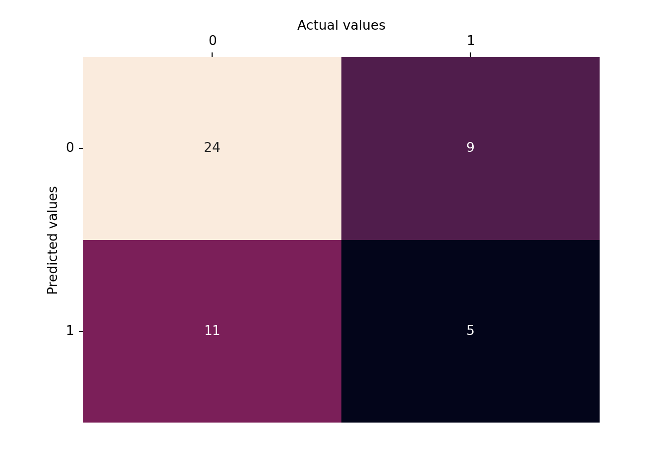
from sklearn.metrics import confusion_matrixcm = confusion_matrix(y_test, y_pred)# visualising the confusion matriximport seaborn as snsax = sns.heatmap(cm, annot=True, fmt="d", cbar=False)ax.xaxis.tick_top()ax.xaxis.set_label_position('top')ax.set_xlabel('Actual values')ax.set_ylabel('Predicted values')plt.yticks(rotation=0);
The model seems to have a higher number of false negatives and false positives, indicating that it may not be very accurate at correctly classifying smokers in this particular dataset.
5.3.5 Validation
The validation is also very similar to what we performed with linear regression. We want to look at the cross validation score and we will have 5 CV folds. We will use accuracy for the scoring parameter but any of the evaluation metrics we looked at above can be used.
# cross validationacc = cross_val_score(clf, X, y, cv =5, scoring='accuracy')print(acc)
The classification model can be tuned by tweaking the following parameters: - criterion: gini/entropy - max_depth: specifies maximum depth of the tree. A deeper tree can model more complex patterns but might lead to overfitting. However, a shallow tree might underfit the data. - splitter: Determines how the nodes are split. The ‘best’ splitter considers all possible splits, while ‘random’ chooses the best random split. ‘Best’ is more computationally intensive but often more accurate, whereas ‘random’ is faster and suitable for large datasets. - min_samples_leaf: The minimum number of samples a leaf node must have. Increasing this number can smooth the model. - min_samples_split: Defines the minimum number of samples required to split an internal node. Higher values prevent the model from learning too specific patterns, hence guarding against overfitting. - max_features: The number of features to consider when looking for the best split. Can be used to limit overfitting and improve performance, especially in cases where not all features are equally important - class_weight: Useful for imbalanced datasets. It assigns a higher penalty to misclassifying the minority class. This can be set to ‘balanced’ to automatically adjust weights inversely proportional to class frequencies.
In a Jupyter environment, please rerun this cell to show the HTML representation or trust the notebook. On GitHub, the HTML representation is unable to render, please try loading this page with nbviewer.org.
Grid Search is a technique for tuning machine learning models by systematically evaluating all possible combinations of algorithm parameters specified in a grid. While it is effective, it can be computationally intensive, especially for large datasets or when dealing with a vast parameter space.
The primary advantage of Grid Search is its ability to thoroughly search through multiple dimensions of parameter space, but the trade-off is the computational cost and time, especially when the number and range of hyperparameters increase.
# Set up the hyperparameter grid to tuneparam_grid = {'max_depth': [None, 10, 20, 30, 40, 50],'min_samples_split': [2, 5, 10],'min_samples_leaf': [1, 2, 4],'criterion': ['gini', 'entropy'],'class_weight': [None, 'balanced'],'splitter': ['best', 'random']}
In a Jupyter environment, please rerun this cell to show the HTML representation or trust the notebook. On GitHub, the HTML representation is unable to render, please try loading this page with nbviewer.org.
# Retrain the model with the best hyperparametersbest_model = grid_search.best_estimator_# Predicting the Test set resultsy_pred = best_model.predict(X_test)# accuracyaccuracy_score(y_test, y_pred)
0.673469387755102
5.4 Probability predictions and feature importance
So far, the predictions we’ve got were the names of the classes - either smoker/non-smoker, or female/male. The model gave us a final decision based on one of these classes, but what if we wanted to perform this decision based on the probabilities of each class instead?
Probabilities give you more insight than just a simple class label. For example, if you’re predicting whether someone is a smoker or non-smoker, a probability close to 50% means the model is uncertain. This is much more informative than just saying ‘smoker’ or ‘non-smoker’.
In fields like finance or insurance, knowing the probability can help assess risk more effectively. Like, what’s the chance someone will default on a loan? A probability gives a more nuanced risk profile than a simple ‘will default’ / ‘won’t default’.
# predict_proba() predicts class probabilities of the sample Xy_predict_proba = clf.predict_proba(X_test)y_predict_proba[:20]
This outputs an array where we get the probability predictions for all the rows in X_test. The first number shows the probability of the value being in the first class, and the second number shows the probability of the value being in the second class.
# If you're not sure which class comes first, useclf.classes_
array(['No', 'Yes'], dtype=object)
We can also use feature_importance_ to work out which are the most important features out of the ones we selected. This will return an array, of which the values inside add up to 1, and and indicates how important that feature is for making predictions with the model. The higher the number, the more important the feature.
clf.feature_importances_
array([0.50046839, 0. , 0.49953161])
These can be added into a dataframe to see which features the values in the array correspond to.
     features  importance
0  total_bill    0.500468
1         tip    0.000000
2        size    0.499532
5.5 Model evaluation: trade-offs
When we talk about trade-off, we are referring to the balance or compromise between different aspects of model performance and evaluation. One such trade-off is the Precision-Recall Trade-off:
Precision is the proportion of positive identifications that were actually correct. A model with high precision doesn’t label negative samples as positive too often.
Recall (or Sensitivity) is the proportion of actual positives that were identified correctly. A model with high recall captures a large proportion of positive samples.
Increasing precision typically reduces recall and vice versa, especially in imbalanced datasets.
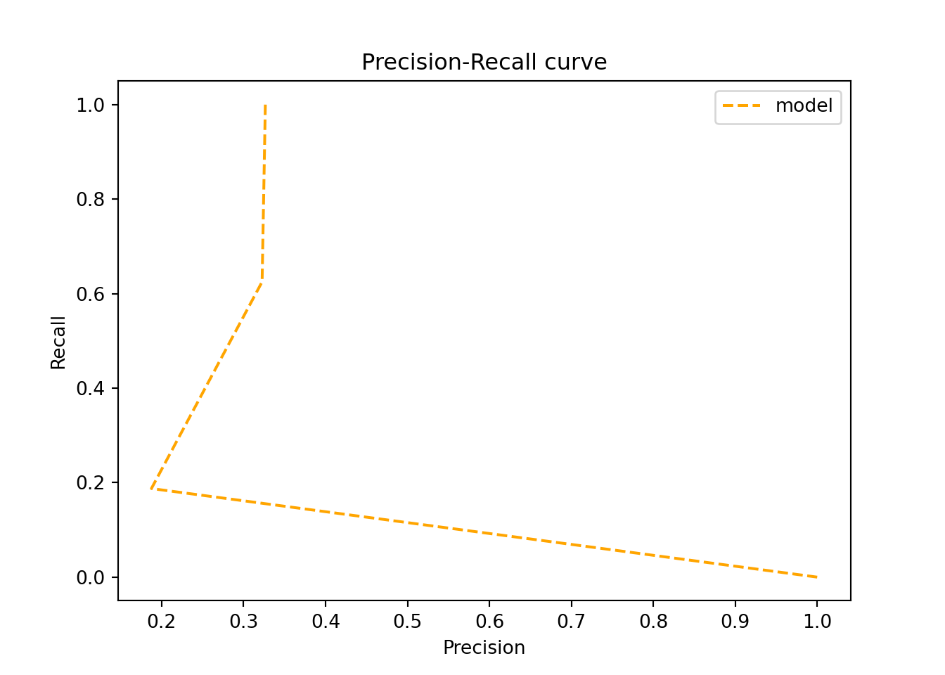
5.5.1 Precision-Recall Curve
from sklearn.metrics import precision_recall_curve# define precision, recall, and thresholdprecision, recall, threshold = precision_recall_curve(y_test, y_predict_proba[:, 1], # all the rows, but only the smokers column pos_label ='Yes') # we want to identify the smokers
# add this to a dataframepr_df = pd.DataFrame([precision[:-1], recall[:-1], threshold]).transpose()pr_df.columns = ['precision', 'recall', 'threshold']pr_df
# visualise into a precision-recall curveplt.plot(precision, recall, linestyle='--',color='orange', label='model')plt.title('Precision-Recall curve')plt.xlabel('Precision')plt.ylabel('Recall')plt.legend(loc='best')
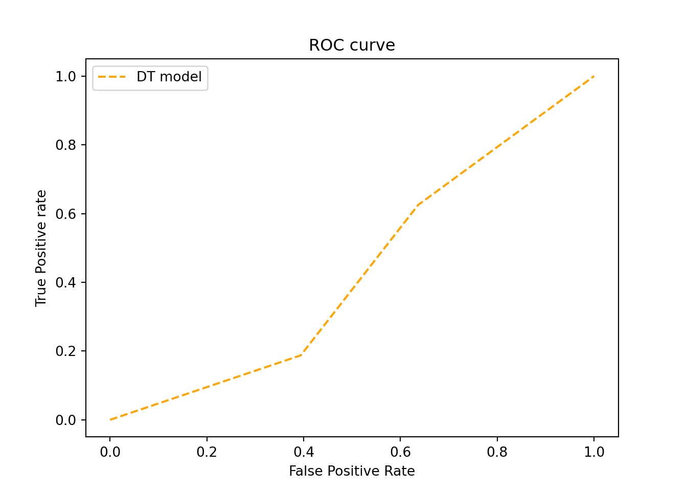
5.5.2 ROC - AUC
We can calculate the ROC AUC score which tells us the chance that the model will be able to distinguish between the positive class and negative class. The ROC AUC score is particularly useful for evaluating models on imbalanced datasets, where the number of instances of one class significantly outweighs the other. It’s less sensitive to this imbalance than other metrics like accuracy.
from sklearn.metrics import roc_auc_scoreroc_auc_score(y_test, y_predict_proba[:, 1])
0.43087121212121215
5.5.2.1 ROC Curve
ROC Curve: This is a graphical representation of the performance of a classification model. It plots two parameters:
True Positive Rate (TPR), also known as Recall or Sensitivity, on the Y-axis. TPR = True Positives / (True Positives + False Negatives).
False Positive Rate (FPR) on the X-axis. FPR = False Positives / (False Positives + True Negatives).
As the classification threshold changes (i.e., the probability at which you decide to classify a sample as positive or negative), the TPR and FPR change, creating a curve.
The area under the curve is equal to the ROC-AUC score.
5.5.3 Evaluation Metrics for Multiclass Classification
Precision and recall require an additional parameter: average.
In a multi-class classification problem, such as predicting species of penguins, you might calculate recall for each class separately. The “average” parameter determines how these individual recall scores are combined into a single metric.
average='micro': Calculate metrics globally by counting the total true positives, false negatives, and false positives. This is useful if you want to weight each instance or prediction equally.
average='macro': Calculate metrics for each label, and find their unweighted mean. This does not take label imbalance into account, so all classes are considered equally important.
average='weighted': Calculate metrics for each label, and find their average, weighted by the number of true instances for each label. This takes label imbalance into account, giving more weight to larger classes.
average='samples': Calculate metrics for each instance, and find their mean (only meaningful for multilabel classification where this differs from accuracy_score).
average=None: The recall scores for each class are returned as an array without averaging.
For a balanced dataset where each class is equally important, ‘macro’ averaging would be appropriate. For an imbalanced dataset, where you care about performance across all instances equally, ‘micro’ might be better. If the class distribution is imbalanced and you want to weight the recall score by the class size, ‘weighted’ averaging should be used.
Documentation for recall: https://scikit-learn.org/stable/modules/generated/sklearn.metrics.recall_score.html
5.6 Ensembles
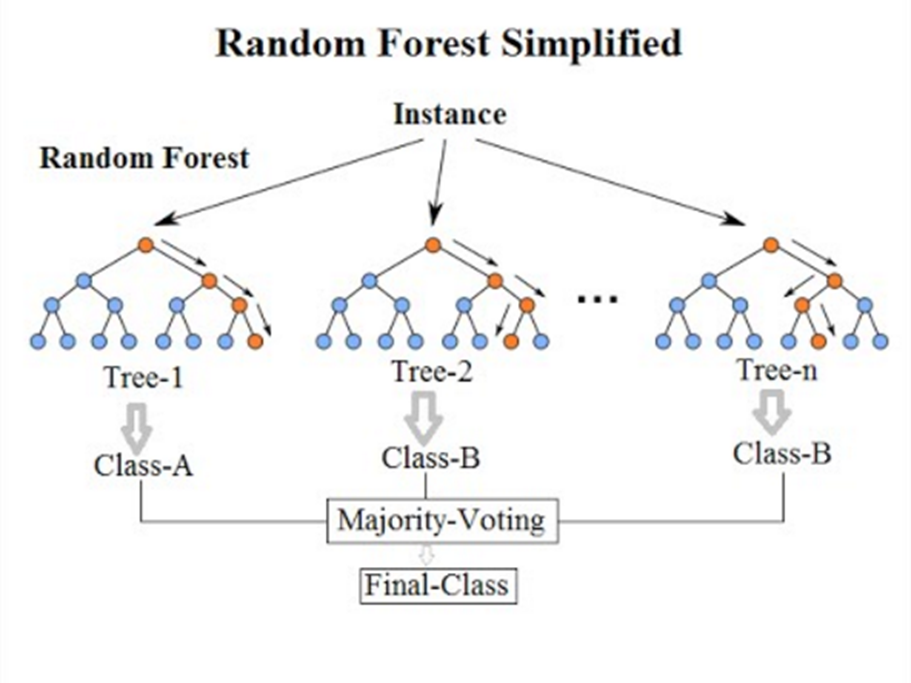
5.6.1 Random Forest - an ensemble of decision trees
Random Forest is a powerful ensemble learning method where the same dataset is used to train multiple decision trees. However, it introduces randomness in two ways: - Each tree in the forest is built from a random sample of the data. - At each split in the tree, a random subset of the features is considered.
5.6.2 Training with Random Forest
Imagine we have a Random Forest consisting of 100 trees. Here’s what happens: - Each decision tree in the Random Forest selects a random subset of features to split the data on during training. - This means that each tree is exposed to different aspects of the data, based on the features it is trained on. - In datasets with many features, say 50 or more, the difference in decision-making between a single decision tree classifier and a Random Forest classifier becomes more pronounced.
5.6.3 Prediction and Voting Mechanism
Each decision tree, trained on different features, will output its own class prediction.
These predictions are then aggregated through a majority voting system.
For example, if we’re classifying penguins and the majority of trees predict a specific penguin is female, then the ensemble will classify it as female.
5.6.4 Advantages of Random Forest
Random Forest pools the expertise of multiple trees, often leading to better accuracy.
Feature selection for predictions is automated with libraries such as scikit-learn, enhancing efficiency.
The model is less prone to overfitting due to the inherent randomness in its design.
5.6.5 Potential Drawbacks
Training time increases with the size of the dataset, which may not be ideal for time-sensitive applications or extremely large datasets.
To implement this with our data, we first need to import the random forest classifier.
from sklearn.ensemble import RandomForestClassifier
The random state is essential here as it controls the randomness of the sample - there is a lot of randomness in a random forest classifier, but we need to have the SAME randomness.
# set up instance of the modelrf = RandomForestClassifier(random_state =1990)# fit the model to the datarf.fit(X_train, y_train)
RandomForestClassifier(random_state=1990)
In a Jupyter environment, please rerun this cell to show the HTML representation or trust the notebook. On GitHub, the HTML representation is unable to render, please try loading this page with nbviewer.org.
print("test data accuracy score: ",accuracy_score(y_test, y_predicted))
test data accuracy score: 0.5918367346938775
How do these accuracy scores compare with the baseline decision tree model?
# confusion matrix for the random forest model (training data)conf_mx = confusion_matrix(y_train, y_estimated)ax = sns.heatmap(conf_mx, annot=True, fmt="d", cbar=False)ax.xaxis.tick_top()ax.xaxis.set_label_position('top')ax.set_xlabel('Actual values')ax.set_ylabel('Predicted values')plt.yticks(rotation=0);
# confusion matrix for the random forest model (test data)conf_mx = confusion_matrix(y_test, y_predicted)ax = sns.heatmap(conf_mx, annot=True, fmt="d", cbar=False)ax.xaxis.tick_top()ax.xaxis.set_label_position('top')ax.set_xlabel('Actual values')ax.set_ylabel('Predicted values')plt.yticks(rotation=0);
# Validate the modelacc = cross_val_score(rf, X, y, cv =5, scoring='accuracy')print(acc)
Documentation for Random Forest: https://scikit-learn.org/stable/modules/generated/sklearn.ensemble.RandomForestClassifier.html
Documentation for classification scores: https://scikit-learn.org/stable/modules/model_evaluation.html
5.6.6 Model tuning
The next step will be to tune the model. The baseline random forest model used 100 trees (this is the default value) which were untrimmed. We now have the chance to trim these models which will help with overfitting.
n_estimators - Number of trees in the forest. (int, default 100)
max_features - max number of features considered for splitting a node. ({“auto”, “sqrt”, “log2”}, int or float, default=”auto”)
max_depth - max number of levels in each decision tree. (int, default=None)
min_samples_split - min number of data points placed in a node before the node is split. (int or float, default=2)
min_samples_leaf - min number of data points allowed in a leaf node. (int or float, default=1)
bootstrap - method for sampling data points (with or without replacement)(bool, default=True, if False all the dataset is used to build the trees)
# an example of a random forest classifier with added parametersrf = RandomForestClassifier(random_state =0, n_estimators =500, max_depth =6, class_weight ='balanced')
In a Jupyter environment, please rerun this cell to show the HTML representation or trust the notebook. On GitHub, the HTML representation is unable to render, please try loading this page with nbviewer.org.
# an example of a random forest classifier with added parametersrf2 = RandomForestClassifier(random_state =0, n_estimators =500, max_depth =3, class_weight ='balanced')rf2.fit(X_train,y_train)
In a Jupyter environment, please rerun this cell to show the HTML representation or trust the notebook. On GitHub, the HTML representation is unable to render, please try loading this page with nbviewer.org.
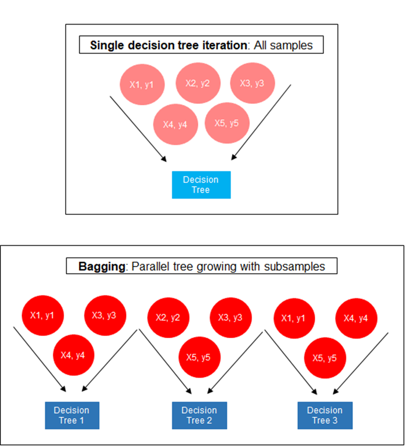
Bagging, short for “Bootstrap Aggregating”, is an ensemble learning technique designed to improve the stability and accuracy of machine learning algorithms. It reduces variance and helps to avoid overfitting. Although it is usually applied to decision tree methods, it can be used with any type of method.
5.7.1 How Bagging Works
Bootstrap Sampling: Multiple subsets of the original dataset are created using bootstrap sampling - that is, sampling with replacement. Each new subset can have the same size as the original dataset.
Model Training: A separate model is trained on each of these bootstrap samples. The learning algorithm is independent and can run in parallel; there is no interaction between the models while they are being trained.
Aggregation of Results: After training, predictions from each model are combined using a simple average (for regression problems) or majority voting (for classification problems).
5.7.2 Advantages of Bagging
Reduces overfitting by averaging out biases.
Can handle high variance in a dataset by training on diverse subsets.
The parallelisable nature of bagging can expedite the training process.
5.7.3 Limitations of Bagging
Bagging can improve accuracy but does not always provide the best bias-variance tradeoff.
The method requires sufficient memory and computational power to train and store multiple models.
A diagram showing how bagging works
To implement this with our data, we first need to import the bagging classifier:
from sklearn.ensemble import BaggingClassifier
# creating an instance of a bagging classifierbagging_clf = BaggingClassifier()
You can then continue to fit and evaluate the model as we have done previously.
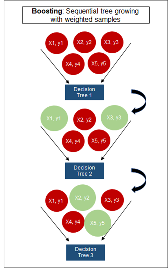
AdaBoost is another ensemble technique, known for its ability to boost the performance of simple models. It works by combining multiple weak classifiers to form a strong classifier. AdaBoost assigns weights to each training instance, which are adjusted as training progresses to force the model to learn harder-to-classify examples.
5.8.1 How AdaBoost Works
Each instance in the training dataset is initially given an equal weight. Then, a weak classifier is trained on the dataset and the errors are evaluated. Instances that are incorrectly predicted by the classifier are given more weight, whereas the weights are decreased for those that are correctly predicted. After several rounds of training classifiers on the reweighted data, the algorithm combines them through a weighted majority vote (for classification problems) to produce the final prediction.
5.8.2 Advantages of AdaBoost
It is often very simple to implement and understand.
Can significantly improve the accuracy of weak classifiers.
Automatically adjusts the weight of misclassified data points.
5.8.3 Limitations of AdaBoost
AdaBoost is sensitive to noisy data and outliers.
It can be prone to overfitting, especially in low-noise scenarios (where the data is very clean, with few, if any, outliers, mislabelled instances, or other anomalies that could mislead the learning algorithm)
To implement this with our data, we first need to import the AdaBoost classifier:
from sklearn.ensemble import AdaBoostClassifierada = AdaBoostClassifier()
You can then continue to fit and evaluate the model as we have done previously.
Gradient Boosting is an ensemble learning technique that builds models in stages. It is a method of converting weak learners into strong learners by focusing on the errors of previous models and improving upon them.
Gradient Boosting involves an iterative approach where each new model incrementally improves upon the previous ones by correcting the errors made by the previous model.
5.9.1 First Iteration
Step 1: The algorithm starts with a base estimator to make initial predictions. The Gradient Boosting classifier then assesses these predictions to identify the errors.
Step 2: A new model is trained to predict these errors, not the actual target variable, effectively learning from the mistakes of the previous model.
5.9.2 Second Iteration
The next model in the sequence focuses on the errors made by the combined predictions of the previous models. It aims to correct these errors, resulting in an improved ensemble.
5.9.3 Subsequent Iterations
This process repeats for a number of iterations (n), each time focusing on the errors of the entire ensemble up to that point.
The final model is a combination of all the weak learners, which can be as simple as decision tree stumps (trees with a single split).
5.10 Learning Rate
An important parameter in Gradient Boosting is the learning rate, which determines the impact of each tree on the final outcome.
A smaller learning rate means that each tree has a smaller corrective impact, requiring more trees to model all the complexities in the data.
Conversely, a higher learning rate allows each tree to have a greater corrective impact, but it also increases the risk of overfitting.
5.11 Gradient Boosting Pros and Cons
Pros - Often provides predictive accuracy that cannot be trumped by other algorithms.
Can handle different types of predictor variables and accommodate missing data.
Cons - Can be computationally expensive due to the sequential nature of boosting.
More prone to overfitting if the data is noisy or the number of iterations is not controlled properly.
The model’s complexity makes it more difficult to interpret than simpler models.
A diagram showing the importance of the learning rate
If the learning rate is too low, the model will take many iterations to converge to the best solution.
The optimal learning rate finds the right balance, achieving convergence without too many iterations.
A learning rate that is too high can cause the model to overshoot the minimum or to diverge, leading to poor performance.
To implement this with our data, we first need to import the GradientBoosting classifier:
from sklearn.ensemble import GradientBoostingClassifiergb_clf = GradientBoostingClassifier()
You can then continue to fit and evaluate the model as we have done previously.
Grid Search is a technique for tuning machine learning models by systematically evaluating all possible combinations of algorithm parameters specified in a grid. While it is effective, it can be computationally intensive, especially for large datasets or when dealing with a vast parameter space.
The primary advantage of Grid Search is its ability to thoroughly search through multiple dimensions of parameter space, but the trade-off is the computational cost and time, especially when the number and range of hyperparameters increase.
In a Jupyter environment, please rerun this cell to show the HTML representation or trust the notebook. On GitHub, the HTML representation is unable to render, please try loading this page with nbviewer.org.
In a Jupyter environment, please rerun this cell to show the HTML representation or trust the notebook. On GitHub, the HTML representation is unable to render, please try loading this page with nbviewer.org.
Random Search CV will train a model with a random sample of hyperparameters. This means that not all the parameters values specified by us will be used.
Using Random Search CV when the sample space, entire range of possible values that each hyperparameter can take is very large(has more than three parameters) is recommended.
In a Jupyter environment, please rerun this cell to show the HTML representation or trust the notebook. On GitHub, the HTML representation is unable to render, please try loading this page with nbviewer.org.
In a Jupyter environment, please rerun this cell to show the HTML representation or trust the notebook. On GitHub, the HTML representation is unable to render, please try loading this page with nbviewer.org.
5.12.3 Choosing Between Grid Search and Random Search
Grid Search: Use when the hyperparameter space is relatively small and computational resources allow for an exhaustive search.
Random Search: Preferable when the hyperparameter space is large and you have a limited computational budget.
5.13 Other Classification Models
More types of classifiers built in scikit learn and their visualizations: https://scikit-learn.org/stable/auto_examples/classification/plot_classifier_comparison.html
5.13.1 KNN (K Nearest Neighbours)
Example: Analysing a dataset containing house prices, aiming to classify them based on how quickly they sell.
Class A (red stars): Houses that sell in under six months.
Class B (green triangles): Houses that take over six months to sell.
The “K” in KNN represents the number of nearest neighbours we consider to determine the class of a new example (a house, in our case).
For instance, with K set to 1, we look for the single nearest data point to our new example. If this nearest neighbour is a Class A house, our new house is predicted to also belong to Class A, indicating it’s likely to sell in under six months.
But what happens when we adjust K? Let’s say we increase K to 3 or even 5. We don’t just consider the single closest neighbour but instead the majority vote among the 3 or 5 nearest neighbours. If, within this selection, there are more Class B houses, our new example will be classified as Class B.
Opting for a smaller K makes our prediction more sensitive to noise in the dataset. In contrast, a larger K, while potentially smoothing out the noise, can lead to higher computational costs and might include neighbours from other classes, diluting the prediction’s accuracy.
A graph showing how a new data point may be classified with KNN
5.13.2 Implementation
from sklearn.neighbors import KNeighborsClassifier# Initialise KNNknn = KNeighborsClassifier(n_neighbors =7)# default n_neighbors = 5# fit model to the dataknn.fit(X_train, y_train)
KNeighborsClassifier(n_neighbors=7)
In a Jupyter environment, please rerun this cell to show the HTML representation or trust the notebook. On GitHub, the HTML representation is unable to render, please try loading this page with nbviewer.org.
KNeighborsClassifier(n_neighbors=7)
# use the fitted model to predict the labels of the test sety_predict = knn.predict(X_test)
# test accuracy scoreaccuracy_score(y_test, y_predict)
0.6326530612244898
# training accuracy scorey_train_estimated = knn.predict(X_train)accuracy_score(y_train, y_train_estimated)
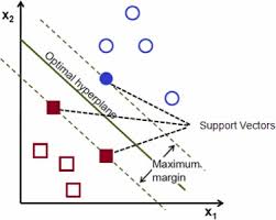
SVM, or Support Vector Machine, is a type of classifier that, despite being classified as such, works as a regression model under the hood. SVM aims to divide datasets into two categories based on a hyperplane that optimally separates the data points.
Hyperplane and Dimensionality - In the context of SVM, a hyperplane is the decision boundary that separates different classes within the dataset. - One-dimensional data (Single Feature): If the dataset is based on a single feature, such as the price of houses, the hyperplane is a straight line that separates houses into two typologies based on their price. - Two-dimensional data (Two Features): With an additional feature, like the surface area of houses, the separation is achieved through a hyperplane in a higher dimension, effectively a “straight plane” that divides the dataset into clusters.
Support Vectors and Margins - Support Vectors: Data points that are closest to the hyperplane and influence its position and orientation. - Margins: The distance between the hyperplane and the nearest data point from either side. Optimal separation is achieved by maximizing this margin.
Kernel Trick - SVM can use different kernels to transform the input space, allowing for the separation of data that is not linearly separable in its original space. - Linear Kernel: Used for linearly separable data, resulting in a straight-line hyperplane. - Polynomial and Radial Basis Function (RBF) Kernels: Enable SVM to create non-linear boundaries, accommodating complex datasets with a free-form hyperplane or polyline, respectively.
from sklearn.svm import SVCsvc = SVC()svc.fit(X_train, y_train)
SVC()
In a Jupyter environment, please rerun this cell to show the HTML representation or trust the notebook. On GitHub, the HTML representation is unable to render, please try loading this page with nbviewer.org.
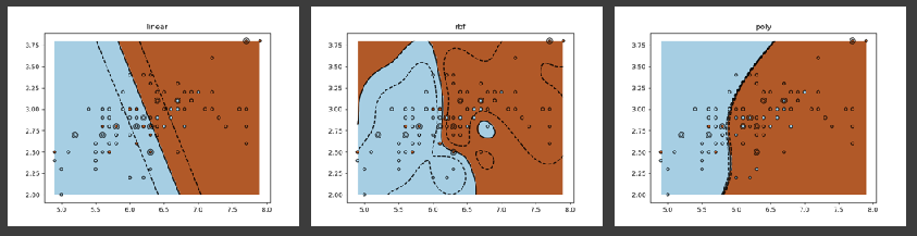
Kernels are functions used to take data as input and transform it into the required form. Different SVM algorithms use different types of kernel functions. The kernel function is what allows SVMs to fit the optimal boundary between the output categories. Different kernels will have different decision boundaries.
Different types of kernels in SVM
Linear Kernel: A linear kernel can be used when the data is linearly separable, meaning when a single straight line can separate the classes.
Polynomial Kernel: It is popular in image processing.
Gaussian kernel: It is a general-purpose kernel; used when there is no prior knowledge about the data. Equation is:
Radial Basis Function (RBF) Kernel: It is a general-purpose kernel; used when there is no prior knowledge about the data.
Sigmoid Kernel: The sigmoid kernel has a similar form to the activation function used in neural networks. It is equivalent to a two-layer, perceptron model of the neural network, which makes it useful for neural networks.
6 Clusters
Clustering is about grouping objects, data points, or entities based on their similarities. Imagine you’re in a room full of people. Without knowing anyone, you might start grouping them based on visible characteristics like clothing style, age, or even the types of gadgets they use. In data analysis, clustering helps us understand our data better. By identifying groups or “clusters” within our data, we can start to see how different subsets of our data share common traits. This is useful for:
Pattern Recognition: Spotting trends and patterns that aren’t immediately obvious.
Data Organisation: Making large datasets more manageable and understandable.
Decision Making: Informing strategic decisions based on the natural groupings within your data.
6.0.1 Types of Clustering
There are several methods to cluster data, but they generally fall into two main categories:
Partitioning Methods: This involves dividing your data into several clusters from the outset. The most famous example is K-means clustering, where ‘K’ represents the number of clusters you want to divide your data into. The algorithm then iterates to group the data into clusters based on the proximity to the center of each cluster.
Hierarchical Clustering: Think of this as organising your data into a family tree of clusters. You start with each data point in its own cluster and then combine clusters step by step, based on their similarity, until all points are in a single cluster or until a certain condition is met.
More clusters here: https://scikit-learn.org/stable/modules/clustering.html
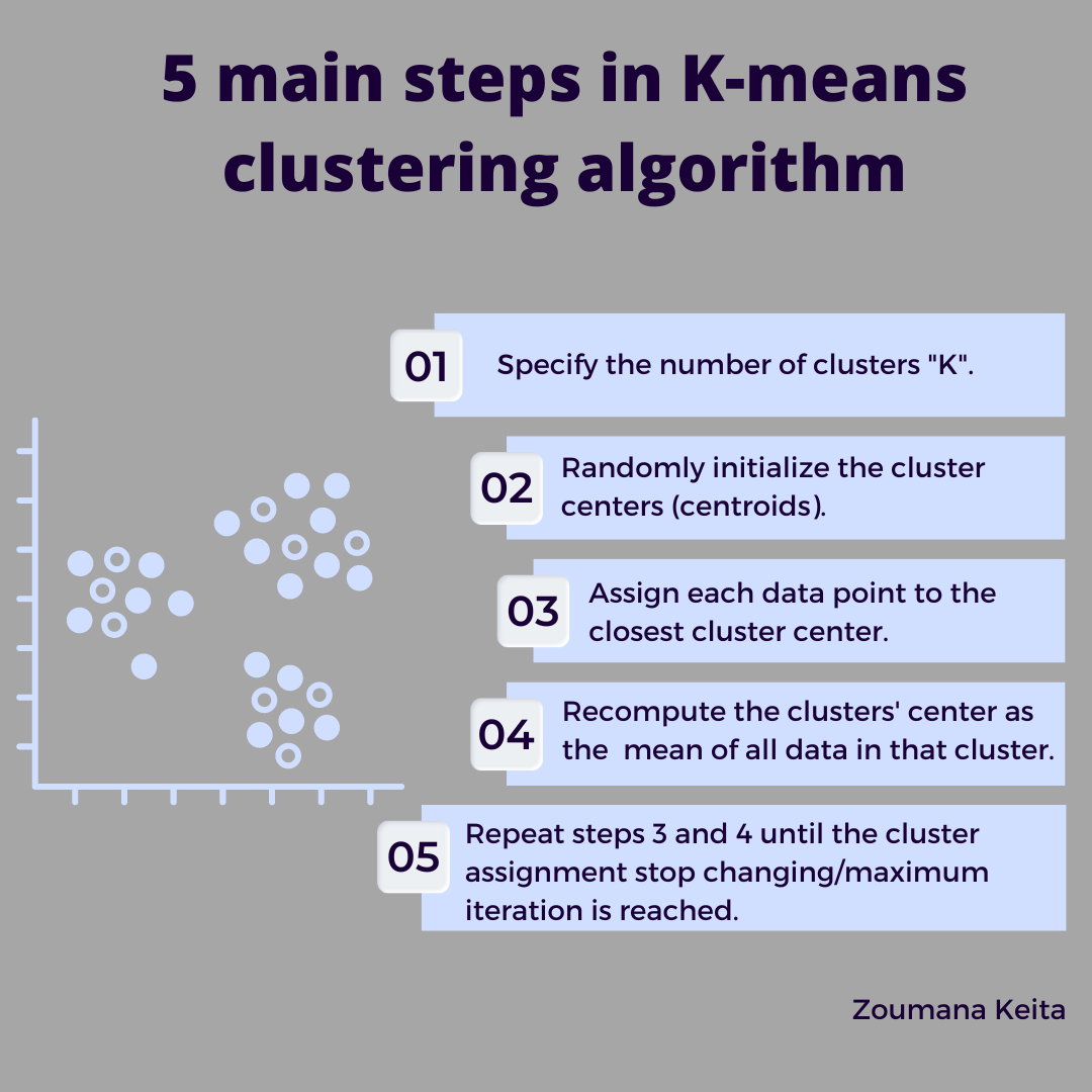
6.0.2 KMeans
K-means is a type of partitioning clustering method. It aims to divide a dataset into ‘K’ distinct clusters based on the features of the data points. The ‘K’ in K-means represents the number of clusters we choose to find in the dataset. Each cluster is defined by its centre, also known as the centroid, which is the average of all the points in the cluster.
Why Use K-Means?
K-means clustering is particularly popular due to its simplicity and efficiency. It’s widely used in a variety of applications, including:
Market Segmentation: Understanding different customer groups to tailor marketing strategies.
Image Compression: Reducing the number of colours that appear in an image to compress it without significantly impacting quality.
Document Clustering: Organising documents into groups of similar topics for easier management and retrieval.
An explanation of the K-Means process
Advantages - K-means is quick and easy to understand, ideal for large datasets and beginners. - Versatility: It’s applicable across various fields, helping uncover hidden patterns in data.
Disadvantages - Determining the right number of clusters (K) in advance can be challenging without prior data insight. - Assumes clusters are spherical and evenly sized, which might not hold for all datasets, potentially affecting accuracy.
6.0.3 Implementation
from sklearn.cluster import KMeans# Standardize the featuresscaler = StandardScaler()features_scaled = scaler.fit_transform(X)
Standardising features ensures all data points are on the same scale, preventing any single feature from dominating due to its larger magnitude. By scaling the data so that each feature has a mean of 0 and a standard deviation of 1, we ensure that the clustering algorithm considers the relative importance of each feature equally, leading to more meaningful and balanced clusters.
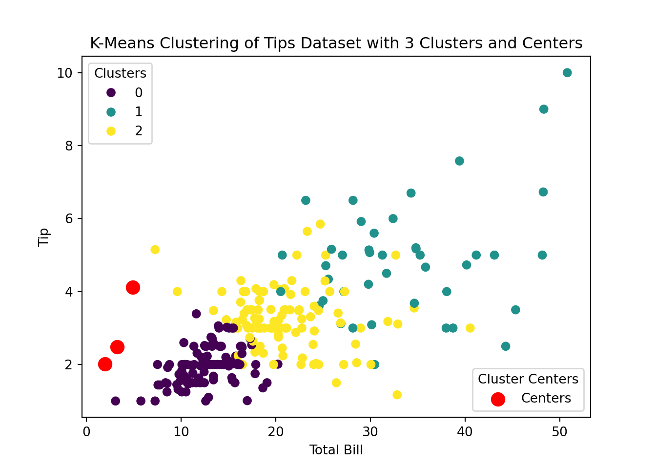
# Plottingfig, ax = plt.subplots()scatter = ax.scatter(tips['total_bill'], tips['tip'], c=tips['cluster'], cmap='viridis', label=tips['cluster'])# Plot cluster centerscenters = scaler.inverse_transform(kmeans.cluster_centers_)centers_scatter = ax.scatter(centers[:, 1], centers[:, 2], s=100, c='red', marker='o', label='Centers')# Add legend with cluster labelslegend1 = ax.legend(*scatter.legend_elements(), title="Clusters")ax.add_artist(legend1)# Add a legend for the centersplt.legend(handles=[centers_scatter], loc='lower right', title="Cluster Centers")# Add labels and titleax.set_xlabel('Total Bill')ax.set_ylabel('Tip')ax.set_title('K-Means Clustering of Tips Dataset with 3 Clusters and Centers')plt.show()
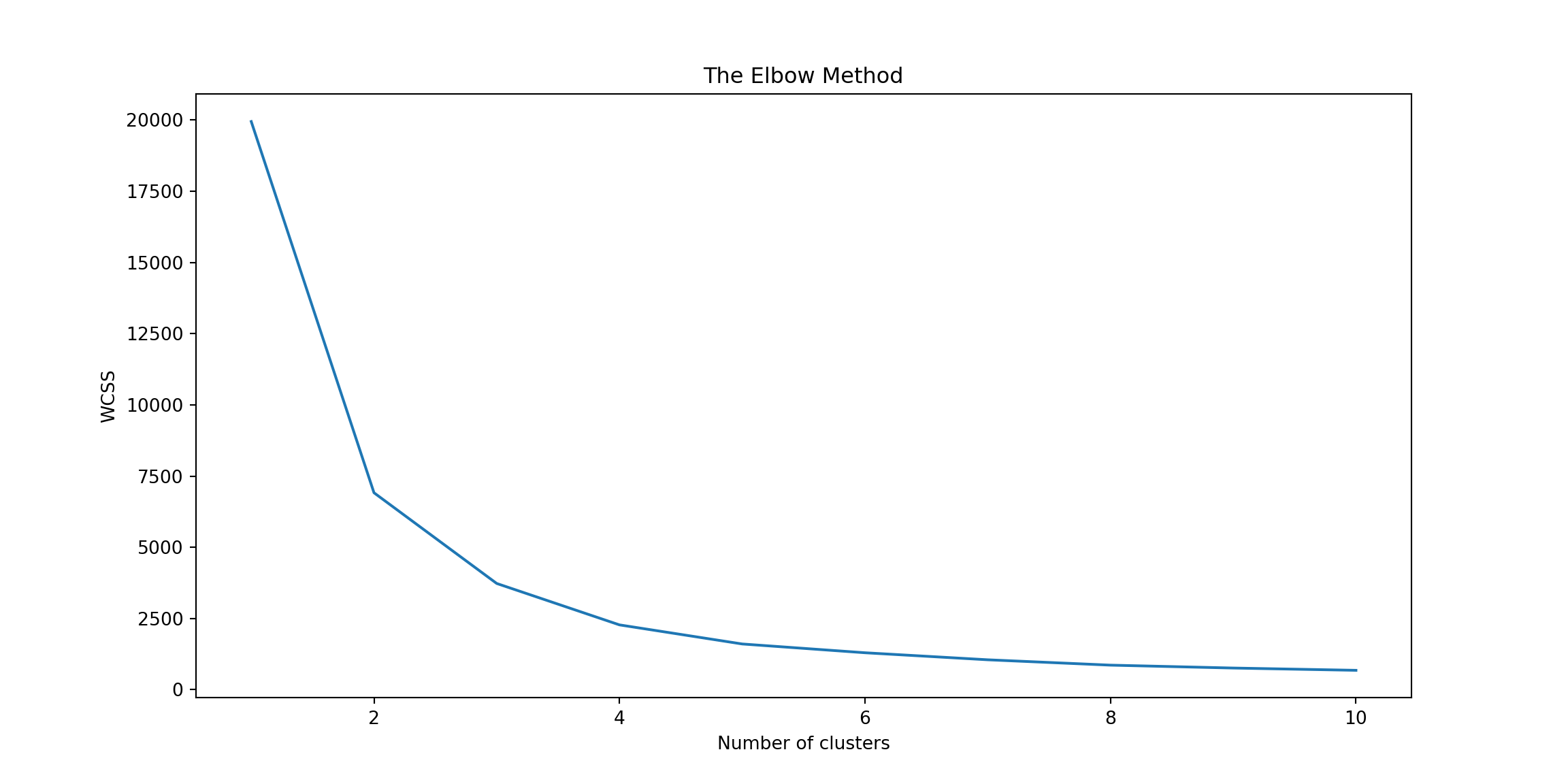
6.0.4 The Elbow Method
Choosing the number of clusters in K-means clustering can significantly affect the results. The Elbow Method is a technique to determine the optimal cluster count. It involves plotting the within-cluster sum of square (WSS), to their closest cluster centre, against the number of clusters. You look for the “elbow” point where the decrease in the sum of squared distances starts to slow down, suggesting that adding more clusters doesn’t significantly improve the fit.
wcss = []for i inrange(1, 11): # Test 1 to 10 clusters kmeans = KMeans(n_clusters=i, init='k-means++', max_iter=300, n_init=10, random_state=0) kmeans.fit(X) wcss.append(kmeans.inertia_)
KMeans(n_clusters=10, n_init=10, random_state=0)
In a Jupyter environment, please rerun this cell to show the HTML representation or trust the notebook. On GitHub, the HTML representation is unable to render, please try loading this page with nbviewer.org.
KMeans(n_clusters=10, n_init=10, random_state=0)
plt.figure(figsize=(12, 6))plt.plot(range(1, 11), wcss)plt.title('The Elbow Method')plt.xlabel('Number of clusters')plt.ylabel('WCSS') # Within-cluster sum of squaresplt.show()
6.1 Logistic Regression
Logistic regression is a statistical model used for binary classification tasks, where the goal is to separate data points into one of two categories. It works by predicting the probability that a given data point belongs to one of the categories, based on its features.
Logistic regression applies a logistic function to a linear combination of features to predict the probability of the target variable being one class or the other. The logistic function, also known as the sigmoid function, ensures that the output of the model is bounded between 0 and 1, which makes it interpretable as a probability.
The coefficients of the linear combination (the model parameters) are typically learned from the training data using a method called maximum likelihood estimation. The logistic regression model finds the set of coefficients that makes the observed classes in the training data most probable.
6.2 Advantages
Logistic regression is straightforward to implement, interpret, and is computationally not intensive.
It provides probabilities for predictions, offering more information than just a binary outcome.
6.3 Disadvantages
It can underperform on more complex or non-linear relationships without feature engineering or transformation.
6.4 When is Logistic Regression Used?
Logistic regression is ideal for problems where the outcome is binary, such as spam detection (spam or not spam), medical diagnosis (sick or healthy), and credit scoring (default or not default).
It is often used as a baseline because of its simplicity and because it can serve as a stepping stone to more complex models and analyses.
It can also be used in multiclass classification problems, though this requires extending the binary logistic regression model to a multinomial one.
# defining target and featuresy = tips['sex']X = tips[['size', 'total_bill', 'tip']]# train test splitX_train, X_test, y_train, y_test = train_test_split(X, y, test_size =0.3, random_state =2024 )
from sklearn.linear_model import LogisticRegression# initialise logistic regression modeLlogreg = LogisticRegression()# fit model to datalogreg.fit(X_train, y_train)
LogisticRegression()
In a Jupyter environment, please rerun this cell to show the HTML representation or trust the notebook. On GitHub, the HTML representation is unable to render, please try loading this page with nbviewer.org.
LogisticRegression()
# test accuracy scorey_predict = logreg.predict(X_test)accuracy_score(y_test, y_predict)
from sklearn.linear_model import LinearRegressionmodel = LinearRegression()model.fit(X_train, y_train)
LinearRegression()
In a Jupyter environment, please rerun this cell to show the HTML representation or trust the notebook. On GitHub, the HTML representation is unable to render, please try loading this page with nbviewer.org.
LinearRegression()
model.score(X_train, y_train)
0.5925597385143913
model.score(X_test, y_test)
0.6351815032929773
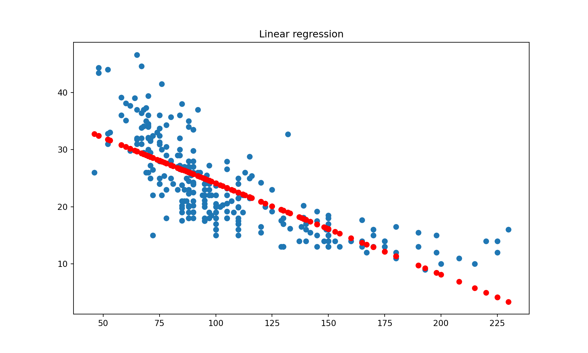
y_train_estimated = model.predict(X_train)
plt.figure(figsize = (10, 6))plt.title('Linear regression')plt.scatter(X_train, y_train)plt.scatter(X_train, y_train_estimated, c ='red')
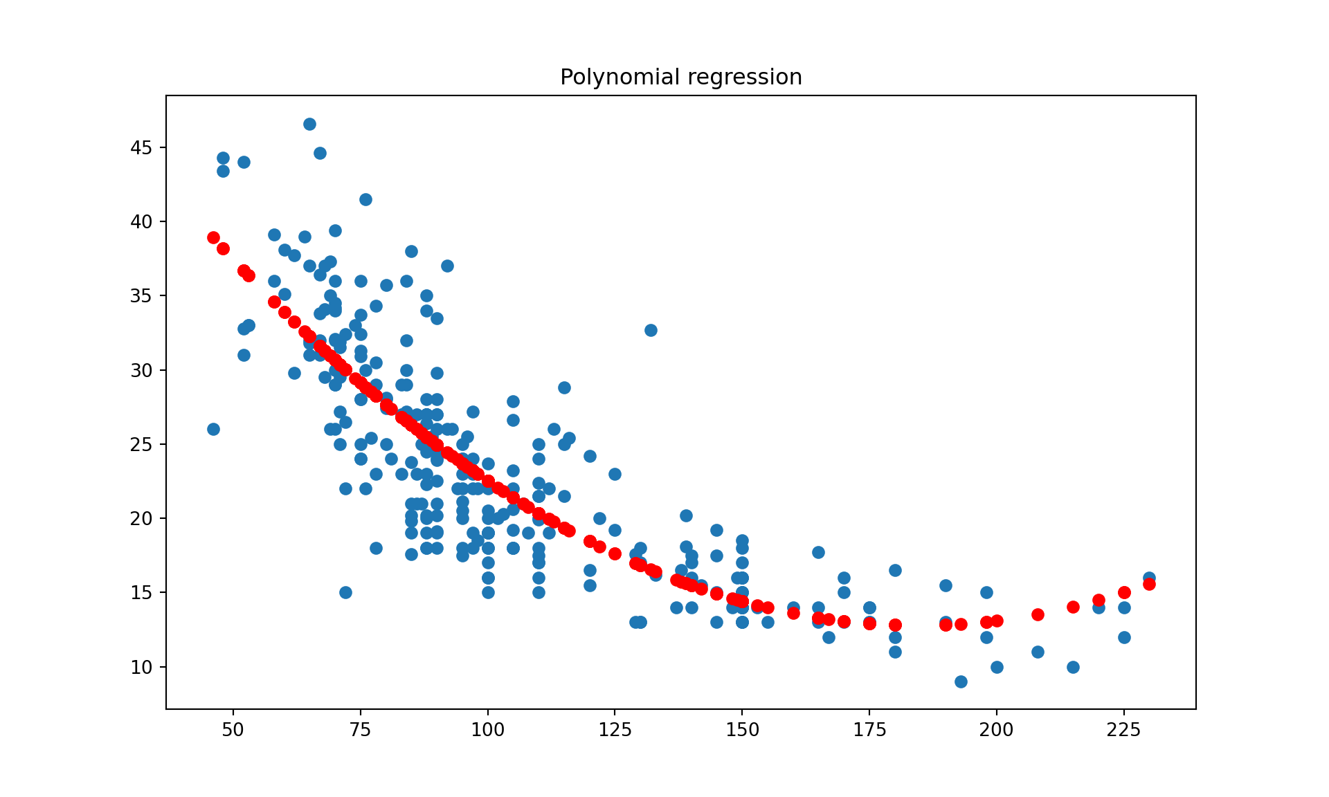
6.5.2 Polynomial Regression - cars dataset
from sklearn.preprocessing import PolynomialFeaturesy = mpg['mpg']X = np.array(mpg[['horsepower']]) # feature matrix# Create a PolynomialFeatures object with degree 2 to capture squared termspoly = PolynomialFeatures(degree=2, include_bias=False)
degree=2: This parameter indicates that you want to transform your input features into all polynomial features of degree 2. In the case of a single feature (like ‘horsepower’), this means you will get two features: the original feature and the square of that feature (i.e., ‘horsepower’ and ‘horsepower’ squared).
include_bias=False: This parameter determines whether or not to include a bias column – a column where every value is 1 – in the output. This column acts as the intercept term in a linear model. Setting include_bias=False means that this column is not added. In many cases, including when using LinearRegression, the bias (intercept) is automatically included by the estimator, so you don’t need to add it manually.
# Fit and transform the features into polynomial featurespoly_features = poly.fit_transform(X.reshape(-1, 1))# train test splitX_train, X_test, y_train, y_test = train_test_split(poly_features, y, test_size =0.3, random_state =2022)# Instantiate a LinearRegression modelpoly_reg_model = LinearRegression()# Fit the modelpoly_reg_model.fit(X_train, y_train)
LinearRegression()
In a Jupyter environment, please rerun this cell to show the HTML representation or trust the notebook. On GitHub, the HTML representation is unable to render, please try loading this page with nbviewer.org.
LinearRegression()
# evaluate on training datapoly_reg_model.score(X_train, y_train)
0.6880771261533316
# evaluate on test datapoly_reg_model.score(X_test, y_test)
0.6803854545693289
# Predict the training data's dependent variable using the fitted modely_train_estimated = poly_reg_model.predict(X_train)
# Get the coefficients of the polynomial regression modelpoly_reg_model.coef_
 ## Clean/Investigate the data
 To implement this with our data, we first need to import the random forest classifier.
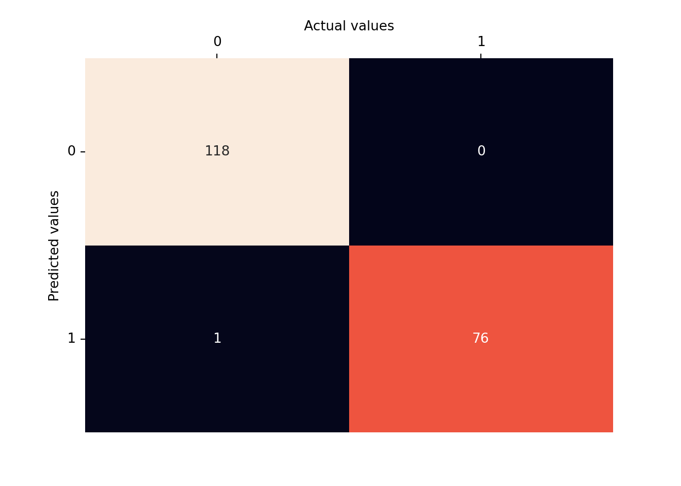
 To implement this with our data, we first need to import the AdaBoost classifier:
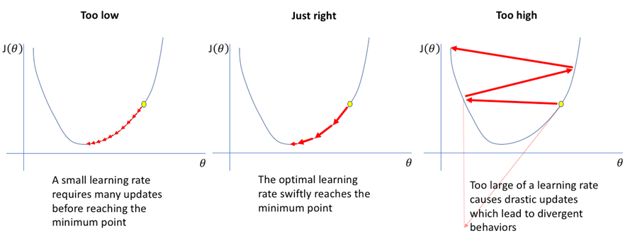


