brk = pd.read_csv('data/MacroTrends_Data_Download_BRK.A.csv', skiprows = 14) # skipping the first 14 rows8 Time Series
8.1 What is time series?
Time series analysis is used for non-stationary data—things that are constantly fluctuating over time or are affected by time. Industries like finance, retail, and economics frequently use time series analysis because currency and sales are always changing. Stock market analysis is an excellent example of time series analysis in action, especially with automated trading algorithms. Likewise, time series analysis is ideal for forecasting weather changes, helping meteorologists predict everything from tomorrow’s weather report to future years of climate change. Examples of time series analysis in action include:
- Weather data
- Rainfall measurements
- Temperature readings
- Heart rate monitoring (EKG)
- Brain monitoring (EEG)
- Quarterly sales
- Stock prices
- Automated stock trading
- Industry forecasts
- Interest rates
There are two main types of time series forecasting.
Univariate Time Series Forecasting:
- Uses only the previous values of the time series to predict its future values.
- Example: t-1, t-2, t-3
Multivariate Time Series Forecasting:
- Uses predictors other than the series (exogenous variables) to forecast.
- Example: to predict the number of bicycle rides: temperature, city, etc.
Example 1
The first dataset we will be using is from this website: https://www.macrotrends.net/stocks/charts/BRK.A/berkshire-hathaway/stock-price-history. It is the stock price history from the last 44 years of a company called Berkshire Hathaway.
brk.head() date open high low close volume
0 1980-03-17 290.0 310.0 290.0 290.0 10000
1 1980-03-18 290.0 290.0 290.0 290.0 0
2 1980-03-19 290.0 310.0 290.0 290.0 20000
3 1980-03-20 290.0 290.0 290.0 290.0 0
4 1980-03-21 290.0 290.0 290.0 290.0 0# information about the dataset
brk.info()<class 'pandas.core.frame.DataFrame'>
RangeIndex: 10498 entries, 0 to 10497
Data columns (total 6 columns):
# Column Non-Null Count Dtype
--- ------ -------------- -----
0 date 10498 non-null object
1 open 10498 non-null float64
2 high 10498 non-null float64
3 low 10498 non-null float64
4 close 10498 non-null float64
5 volume 10498 non-null int64
dtypes: float64(4), int64(1), object(1)
memory usage: 492.2+ KB8.2 Date formatting
As a recap: https://docs.python.org/3/library/datetime.html#strftime-and-strptime-behavior
# converting the date column to the datetime format
brk['date'] = pd.to_datetime(brk['date'], format ='%Y-%m-%d')
brk.info() # note the change of datatype for `date`<class 'pandas.core.frame.DataFrame'>
RangeIndex: 10498 entries, 0 to 10497
Data columns (total 6 columns):
# Column Non-Null Count Dtype
--- ------ -------------- -----
0 date 10498 non-null datetime64[ns]
1 open 10498 non-null float64
2 high 10498 non-null float64
3 low 10498 non-null float64
4 close 10498 non-null float64
5 volume 10498 non-null int64
dtypes: datetime64[ns](1), float64(4), int64(1)
memory usage: 492.2 KB8.3 Time series structure
8.3.1 Cycles
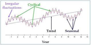
A seasonal pattern exists when a series is influenced by seasonal factors (e.g., the quarter of the year, the month, or day of the week). Seasonality is always of a fixed and known period. Hence, seasonal time series are sometimes called periodic time series.
A cyclic pattern exists when data exhibit rises and falls that are not of fixed period. The duration of these fluctuations is usually of at least 2 years. Think of business cycles which usually last several years, but where the length of the current cycle is unknown beforehand.
Many people confuse cyclic behaviour with seasonal behaviour, but they are really quite different. If the fluctuations are not of fixed period then they are cyclic; if the period is unchanging and associated with some aspect of the calendar, then the pattern is seasonal. In general, the average length of cycles is longer than the length of a seasonal pattern, and the magnitude of cycles tends to be more variable than the magnitude of seasonal patterns.
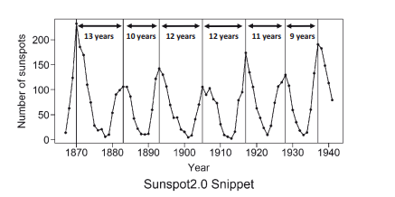
Example 2
# read in sunspots data
sunspots = pd.read_csv('data/sunspots.csv')
sunspots.info()
<class 'pandas.core.frame.DataFrame'>
RangeIndex: 3265 entries, 0 to 3264
Data columns (total 3 columns):
# Column Non-Null Count Dtype
--- ------ -------------- -----
0 Unnamed: 0 3265 non-null int64
1 Date 3265 non-null object
2 Monthly Mean Total Sunspot Number 3265 non-null float64
dtypes: float64(1), int64(1), object(1)
memory usage: 76.7+ KB# convert date column to datetime
sunspots['Date'] = pd.to_datetime(sunspots['Date'])# plotting the time series graph
plt.figure(figsize = (10,5))
plt.plot(sunspots['Date'], # x axis
sunspots['Monthly Mean Total Sunspot Number']) # y axis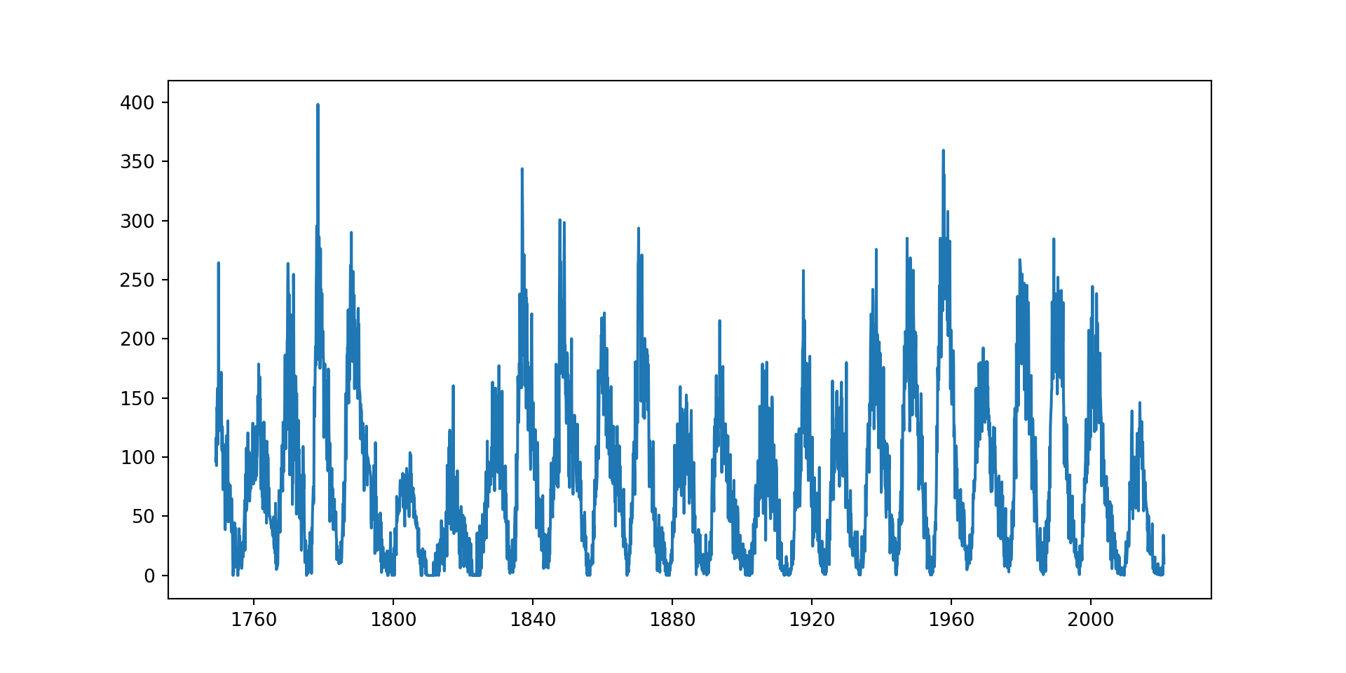
Data that are truly periodic have a behavior that repeats exactly over a fixed time frame.
Example 3
# read in airpass data
airpass = pd.read_csv('data/AirPassengers.csv')
airpass.info()
<class 'pandas.core.frame.DataFrame'>
RangeIndex: 144 entries, 0 to 143
Data columns (total 2 columns):
# Column Non-Null Count Dtype
--- ------ -------------- -----
0 Month 144 non-null object
1 #Passengers 144 non-null int64
dtypes: int64(1), object(1)
memory usage: 2.4+ KBairpass.head() Month #Passengers
0 1949-01 112
1 1949-02 118
2 1949-03 132
3 1949-04 129
4 1949-05 121# convert date column to datetime
airpass['Month'] = pd.to_datetime(airpass['Month'])
airpass.head() Month #Passengers
0 1949-01-01 112
1 1949-02-01 118
2 1949-03-01 132
3 1949-04-01 129
4 1949-05-01 121plt.figure(figsize = (10,5))
plt.plot(airpass['Month'], airpass['#Passengers'], marker = '.')
plt.xlim(left = airpass['Month'][0], right = airpass['Month'][50])(-7670.0, -6150.0)
# plt.axvline(airpass['Month'][12], color = 'red', ls = '--', lw = 0.5)
# plt.axvline(airpass['Month'][24], color = 'red', ls = '--', lw = 0.5)
# plt.axvline(airpass['Month'][36], color = 'red', ls = '--', lw = 0.5)
# plt.axvline(airpass['Month'][48], color = 'red', ls = '--', lw = 0.5)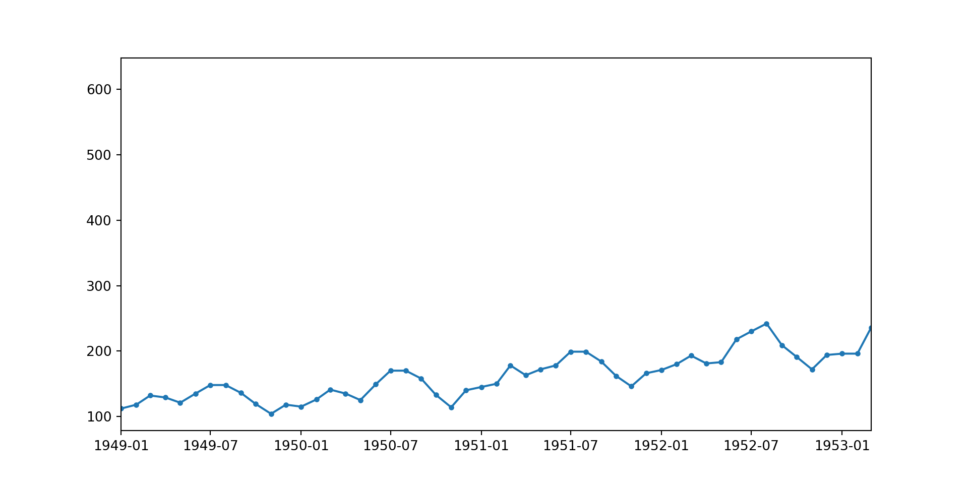
The cyclic behavior of the air passenger data is repeated on an annual basis. This can be better visualised by uncommenting the last four lines in the code cell above.
The data suggests cyclic growth in travel with peaks likely during popular travel months (July, August).
Example 2 showed seasonality over 12 years, and example 3 showed seasonality over 1 year. It’s also possible to have seasonality over a month, for example you might have higher sales at the beginning and end of a month and less sales in the middle of the month. Seasonality could also occur over a week, where a call centre receives more calls on a Monday and less calls on a Friday, and it could also occur over a day, where traffic data shows high volume of cars in the morning and late afternoon, and low volume of cars in the middle of the night.
It’s important to identify the seasonality in your dataset to allow you to recognise the level of granularity needed for your time series model.
8.3.2 Trends
In time series analysis, a trend represents the general direction in which the data moves over time. It is a pattern that persists over a long period, regardless of short-term fluctuations.
a) Linear Trend
This is a straightforward, consistent upward or downward movement at a steady rate. It can be represented by a straight line when plotted on a graph, indicating a constant increase or decrease over time.
b) Exponential Trend
Characterised by data that increases or decreases at an increasingly higher rate. On a graph, this is shown as a curve that moves away from the baseline more and more sharply as time progresses. It’s common in phenomena that spread rapidly, like viral internet content or population growth in certain conditions.
c) Downward Trend
This is a specific type of trend where the data is consistently decreasing over time. It can be linear, with a steady rate of decline, or it can be exponential, with the rate of decline accelerating as time goes on.
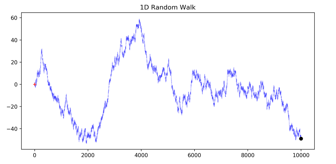
d) Random Walk
This describes a time series that moves up and down seemingly at random, without any long-term direction. This type of data can be challenging to predict and may often require more sophisticated models to understand any underlying structure that isn’t immediately apparent.
8.4 Date as an index
For time series, specifically the ARIMA model, the date needs to be converted to an index.
# before
brk.head()
date open high low close volume
0 1980-03-17 290.0 310.0 290.0 290.0 10000
1 1980-03-18 290.0 290.0 290.0 290.0 0
2 1980-03-19 290.0 310.0 290.0 290.0 20000
3 1980-03-20 290.0 290.0 290.0 290.0 0
4 1980-03-21 290.0 290.0 290.0 290.0 0# after
brk = brk.set_index('date') # specify the column that needs to be indexed
brk.head() open high low close volume
date
1980-03-17 290.0 310.0 290.0 290.0 10000
1980-03-18 290.0 290.0 290.0 290.0 0
1980-03-19 290.0 310.0 290.0 290.0 20000
1980-03-20 290.0 290.0 290.0 290.0 0
1980-03-21 290.0 290.0 290.0 290.0 0This allows us to select specific dates from the index to use for analysis.
# example: select dates from 10th September 2008 to 20th September 2008
brk['2008-09-10':'2008-09-20']
open high low close volume
date
2008-09-10 118500.0 118500.0 117000.0 117000.0 59600
2008-09-11 116200.0 117500.0 115500.0 117500.0 52000
2008-09-12 116700.0 119500.0 116310.0 119500.0 86500
2008-09-15 117000.0 123100.0 115500.0 119900.0 223200
2008-09-16 119000.0 125010.0 118300.0 125000.0 256200
2008-09-17 125000.0 125600.0 122900.0 124800.0 180000
2008-09-18 126000.0 128900.0 121310.0 128010.0 276500
2008-09-19 130000.0 147000.0 127901.0 147000.0 422800Indexing the date also impacts the output of brk.info(). It will give us the range of dates in the dataset.
brk.info()<class 'pandas.core.frame.DataFrame'>
DatetimeIndex: 10498 entries, 1980-03-17 to 2021-10-29
Data columns (total 5 columns):
# Column Non-Null Count Dtype
--- ------ -------------- -----
0 open 10498 non-null float64
1 high 10498 non-null float64
2 low 10498 non-null float64
3 close 10498 non-null float64
4 volume 10498 non-null int64
dtypes: float64(4), int64(1)
memory usage: 750.1 KBExamine the dates from the output above. What is missing? It seems to be the days that correspond with the weekend, which makes sense, as the stock markets aren’t open.
8.5 Filling data gaps
For our model to be effective, we need to have consecutive dates, because the model assumes the points are evenly spaced over time. If not, this implies there are missing values and can distort the model’s understanding.
When forecasting, irregular intervals could lead to misleading results because the model may not correctly attribute changes in the data to either trends or seasonality.
brk[4:6] # can view the missing weekend open high low close volume
date
1980-03-21 290.0 290.0 290.0 290.0 0
1980-03-24 290.0 290.0 270.0 270.0 10000We can use the .resample() method for frequency conversion and resampling of time series data. We can also use .asfreq() which allows the datetime index to have a different frequency, while keeping the same values at the current index.
Link to resample documentation`
brk[4:6].resample('1d').asfreq() # specify 1 day open high low close volume
date
1980-03-21 290.0 290.0 290.0 290.0 0.0
1980-03-22 NaN NaN NaN NaN NaN
1980-03-23 NaN NaN NaN NaN NaN
1980-03-24 290.0 290.0 270.0 270.0 10000.0Now, the missing dates have been added, but we are missing data for the four columns in the dataset.
First we will apply the above function to the entire dataset.
# apply .resample() to whole dataset
brk_resampled = brk.resample('1d').asfreq()
brk_resampled open high low close volume
date
1980-03-17 290.00 310.00 290.00 290.0 10000.0
1980-03-18 290.00 290.00 290.00 290.0 0.0
1980-03-19 290.00 310.00 290.00 290.0 20000.0
1980-03-20 290.00 290.00 290.00 290.0 0.0
1980-03-21 290.00 290.00 290.00 290.0 0.0
... ... ... ... ... ...
2021-10-25 435962.98 437144.50 433064.07 436401.0 1793.0
2021-10-26 437165.12 439849.99 435446.02 437890.0 1902.0
2021-10-27 437526.91 439229.22 433050.00 433050.0 3228.0
2021-10-28 434702.73 436873.99 432516.47 436249.5 2409.0
2021-10-29 435052.79 436511.89 431713.81 432902.0 2072.0
[15202 rows x 5 columns]We can also plot this data. As we have ‘date’ as an index, we can select any other column and a line plot will be returned.
# plot 'open' over time
brk_resampled['open'].plot(figsize = (30, 10))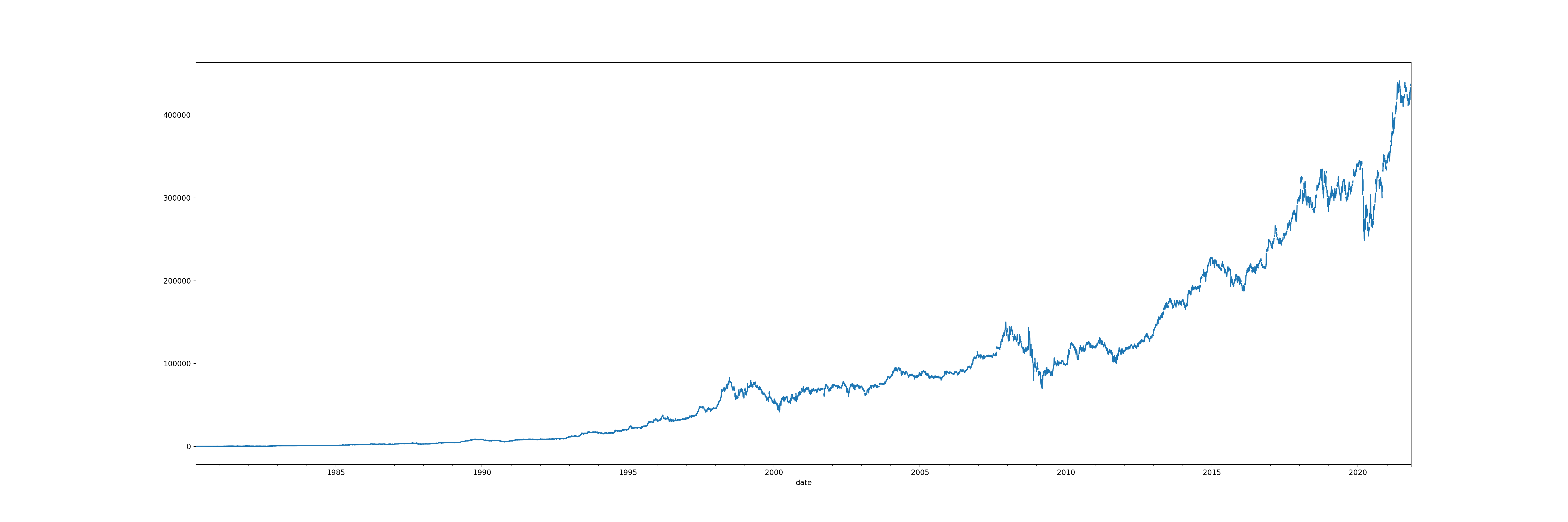
However, double clicking on the graph, we can see there are some gaps - this is where the weekend missing values are. The next step will be to solve this problem.
We have the following options:
.pad()- pads the data with the previous valid values. (forward filling).bfill()- The backward fill will replace NaN values that appeared in the resampled data with the next value in the original sequence. Missing values that existed in the original data will not be modified..ffill()- Forward fill the values.
# resampling with .pad()
brk_filled = brk[4:6].asfreq('1d', method='pad')
brk_filled
open high low close volume
date
1980-03-21 290.0 290.0 290.0 290.0 0
1980-03-22 290.0 290.0 290.0 290.0 0
1980-03-23 290.0 290.0 290.0 290.0 0
1980-03-24 290.0 290.0 270.0 270.0 10000# resampling with .bfill()
brk[4:6].resample('1d').bfill() open high low close volume
date
1980-03-21 290.0 290.0 290.0 290.0 0
1980-03-22 290.0 290.0 270.0 270.0 10000
1980-03-23 290.0 290.0 270.0 270.0 10000
1980-03-24 290.0 290.0 270.0 270.0 10000# using .bfill() on the resampled data
brk_resampled_bfill = brk_resampled.bfill()
brk_resampled_bfill open high low close volume
date
1980-03-17 290.00 310.00 290.00 290.0 10000.0
1980-03-18 290.00 290.00 290.00 290.0 0.0
1980-03-19 290.00 310.00 290.00 290.0 20000.0
1980-03-20 290.00 290.00 290.00 290.0 0.0
1980-03-21 290.00 290.00 290.00 290.0 0.0
... ... ... ... ... ...
2021-10-25 435962.98 437144.50 433064.07 436401.0 1793.0
2021-10-26 437165.12 439849.99 435446.02 437890.0 1902.0
2021-10-27 437526.91 439229.22 433050.00 433050.0 3228.0
2021-10-28 434702.73 436873.99 432516.47 436249.5 2409.0
2021-10-29 435052.79 436511.89 431713.81 432902.0 2072.0
[15202 rows x 5 columns]brk_resampled_bfill.info()<class 'pandas.core.frame.DataFrame'>
DatetimeIndex: 15202 entries, 1980-03-17 to 2021-10-29
Freq: D
Data columns (total 5 columns):
# Column Non-Null Count Dtype
--- ------ -------------- -----
0 open 15202 non-null float64
1 high 15202 non-null float64
2 low 15202 non-null float64
3 close 15202 non-null float64
4 volume 15202 non-null float64
dtypes: float64(5)
memory usage: 712.6 KBbrk_resampled_bfill['open'].plot(figsize=(30, 10), color='red') # new data
brk_resampled['open'].plot(figsize=(30, 10), color='black') # old data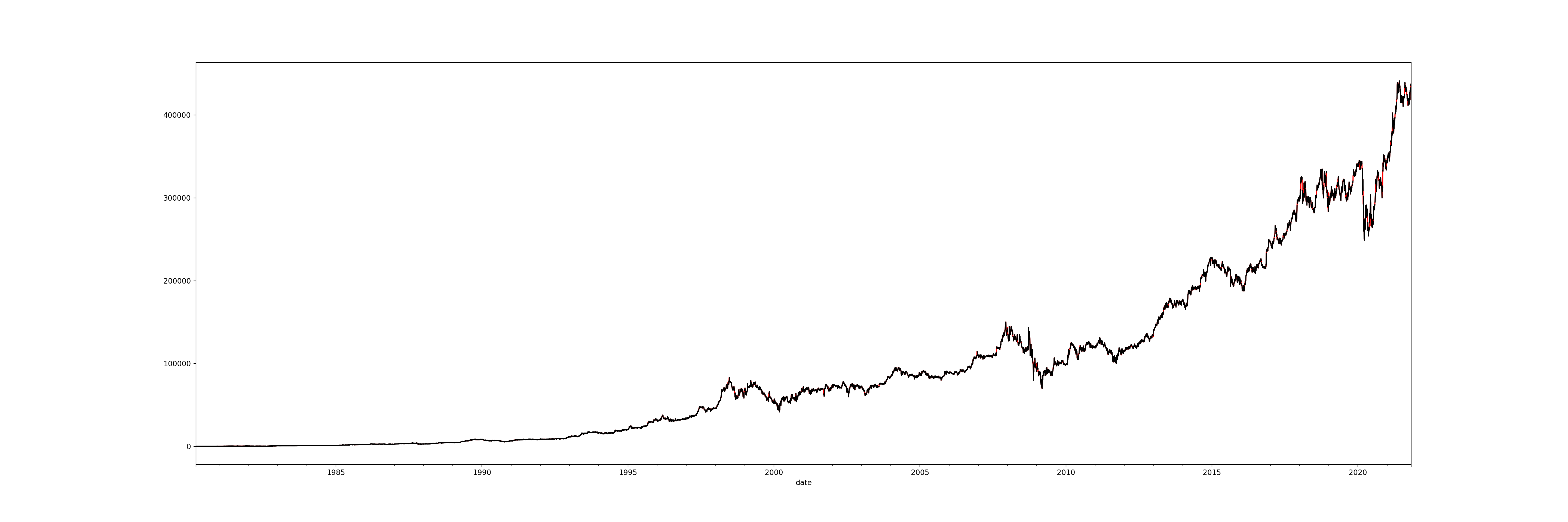
With the red line as the new data and the black line as the old data, we can see that all the gaps have now been covered.
The above is one method we can use to fill in missing values, but there are others which may be more effective.
Ways to fill the missing values:
- with the nearest value
- with the mean, median, most frequent value
- with the predictions of a regressor model (using linear regression to predict the missing values)
- by using the interpolation technique
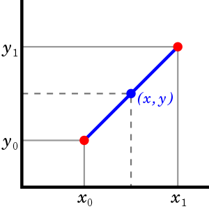
For example, one of the interpolation methods available is linear interpolation. Linear interpolation can be used to input missing data by drawing a straight line between the two points surrounding the missing value(in time series: it looks at prior past value and the next future value to draw a line between them).
A polynomial interpolation will attempt to draw a curved line between the two points.
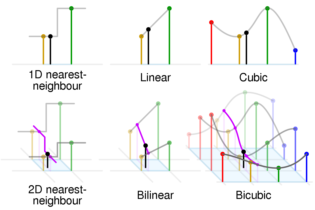
1D Nearest-Neighbour: Assigns the value of the nearest data point to a given x-value without considering the other points. It results in a step-like graph where the interpolated value abruptly changes at the midpoint between neighbouring data points.
Linear: Draws a straight line between two adjacent data points and uses this line to estimate intermediate values. This results in a piecewise linear graph.
Cubic: Uses cubic polynomials to connect the data points, creating a smoother curve than linear interpolation. It takes into account more neighbouring points, which often results in a smoother and more natural-looking curve.
2D Nearest-Neighbour: This technique is an extension of the 1D nearest-neighbour to two dimensions. It assigns the value of the nearest data point to a given (x, y) position, resulting in a block-like pattern in the interpolated surface.
Bilinear: Extends the concept of linear interpolation to two dimensions. It interpolates linearly in both the x and y directions by taking the four nearest grid points to create a smooth surface.
Bicubic: Similar to cubic interpolation in 1D, bicubic interpolation in 2D uses 16 nearby points to estimate the value at a given (x, y) position, resulting in a much smoother surface than both the nearest-neighbour and bilinear methods.
# interpolating the 'open' column using linear
brk_resampled['open_linear'] = brk_resampled['open'].interpolate('linear')

# 'quadratic', 'nearest', 'cubic'brk_resampled_bfill['open'].plot(figsize = (30, 10), color='black') # old data
brk_resampled['open_linear'].plot(figsize = (30, 10), color='red') # new data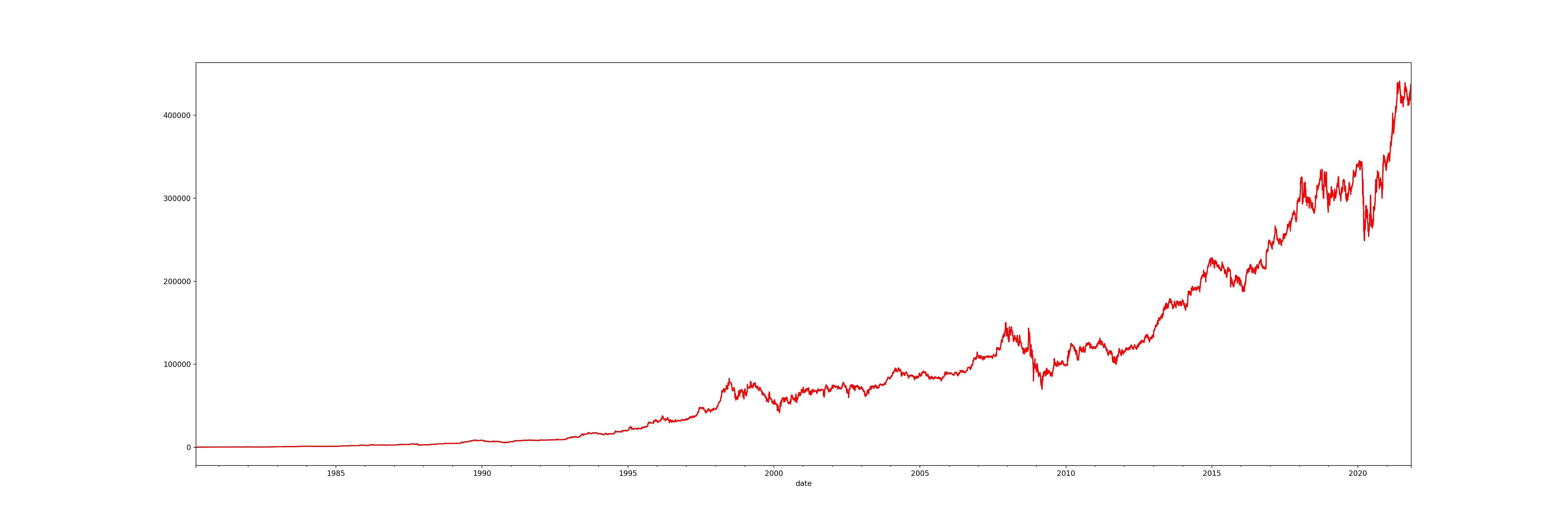
Although there is not a big difference visible, there will be a much larger difference when your dataset has multiple missing values, especially if they are very close to one another.
8.6 Resampling
We can reduce the granularity of the data even further, for example by breaking it down into periods of 6 hours.
# view two days worth of data
brk[2:4]
open high low close volume
date
1980-03-19 290.0 310.0 290.0 290.0 20000
1980-03-20 290.0 290.0 290.0 290.0 0# resample to periods of 6 hours
brk[2:4].resample('6h').asfreq() open high low close volume
date
1980-03-19 00:00:00 290.0 310.0 290.0 290.0 20000.0
1980-03-19 06:00:00 NaN NaN NaN NaN NaN
1980-03-19 12:00:00 NaN NaN NaN NaN NaN
1980-03-19 18:00:00 NaN NaN NaN NaN NaN
1980-03-20 00:00:00 290.0 290.0 290.0 290.0 0.08.7 Downsampling
We can also do the opposite process, to decrease the granularity of the data. Instead of daily data, we may wish to view our data in 1 week bins. This would sum the values of the timestamps falling into a bin.
# view first 2 weeks
brk[:15]
open high low close volume
date
1980-03-17 290.0 310.0 290.0 290.0 10000
1980-03-18 290.0 290.0 290.0 290.0 0
1980-03-19 290.0 310.0 290.0 290.0 20000
1980-03-20 290.0 290.0 290.0 290.0 0
1980-03-21 290.0 290.0 290.0 290.0 0
1980-03-24 290.0 290.0 270.0 270.0 10000
1980-03-25 270.0 270.0 270.0 270.0 0
1980-03-26 270.0 270.0 270.0 270.0 0
1980-03-27 270.0 270.0 270.0 270.0 0
1980-03-28 270.0 270.0 270.0 270.0 0
1980-03-31 270.0 280.0 260.0 260.0 10000
1980-04-01 260.0 280.0 260.0 260.0 30000
1980-04-02 260.0 260.0 260.0 260.0 0
1980-04-03 260.0 280.0 260.0 260.0 10000
1980-04-07 265.0 285.0 265.0 265.0 10000We can use the .resample() method, specifying 1 week. Instead of asfreq(), we use.sum()` to add the values.
# resample on just one column (volume)
brk['volume'].resample('1w').sum()
date
1980-03-23 30000
1980-03-30 10000
1980-04-06 50000
1980-04-13 120000
1980-04-20 70000
...
2021-10-03 4989
2021-10-10 6059
2021-10-17 6360
2021-10-24 7283
2021-10-31 11404
Freq: W-SUN, Name: volume, Length: 2172, dtype: int64
<string>:2: FutureWarning: 'w' is deprecated and will be removed in a future version, please use 'W' instead.8.8 Exploratory Data Analysis
# select the 'open' column as a series
series = brk['open']
# descriptive statistics about the dataset
series.describe()count 10498.000000
mean 92531.835852
std 101720.441234
min 245.000000
25% 7556.250000
50% 68900.000000
75% 123703.750000
max 441063.000000
Name: open, dtype: float64Things to pay attention to:
- The large standard deviation and the size of the first and third quantiles suggest that the data is widely spread around the mean.
- The mean and median(50%) are not equal. The mean is higher, indicating there may be some large outliers.
- There are 10498 data points.
8.8.1 Plotting
Line plot
# plotting the 'open' column as a time series
brk['open'].plot(figsize = (20, 7))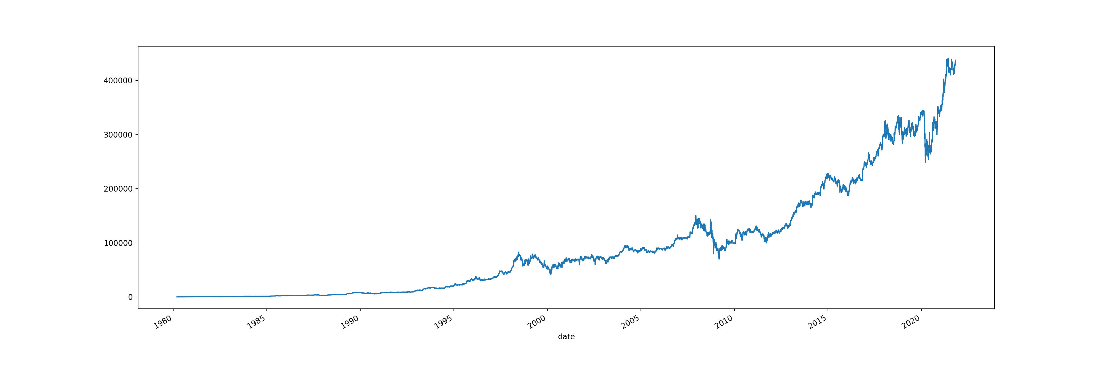
However this just demonstrates the time series graph for one column. By using .plot() on the entire dataframe, we can plot each column on the same graph, with a legend for each column.
# plotting entire dataset
brk.plot(figsize = (20, 10))
Sometimes this can be useful because you might want to compare different variables across the same period of time. However, in this case it isn’t too useful as the graph is not overly readable. We can also split them into multiple subplots to make it more readable.
plt.style.use('default')
# plt.style.use('fivethirtyeight')
brk.plot(figsize = (20,10), subplots = True);


# styles: 'fivethirtyeight', 'dark_background', 'seaborn-dark', 'tableau-colorblind10', 'default'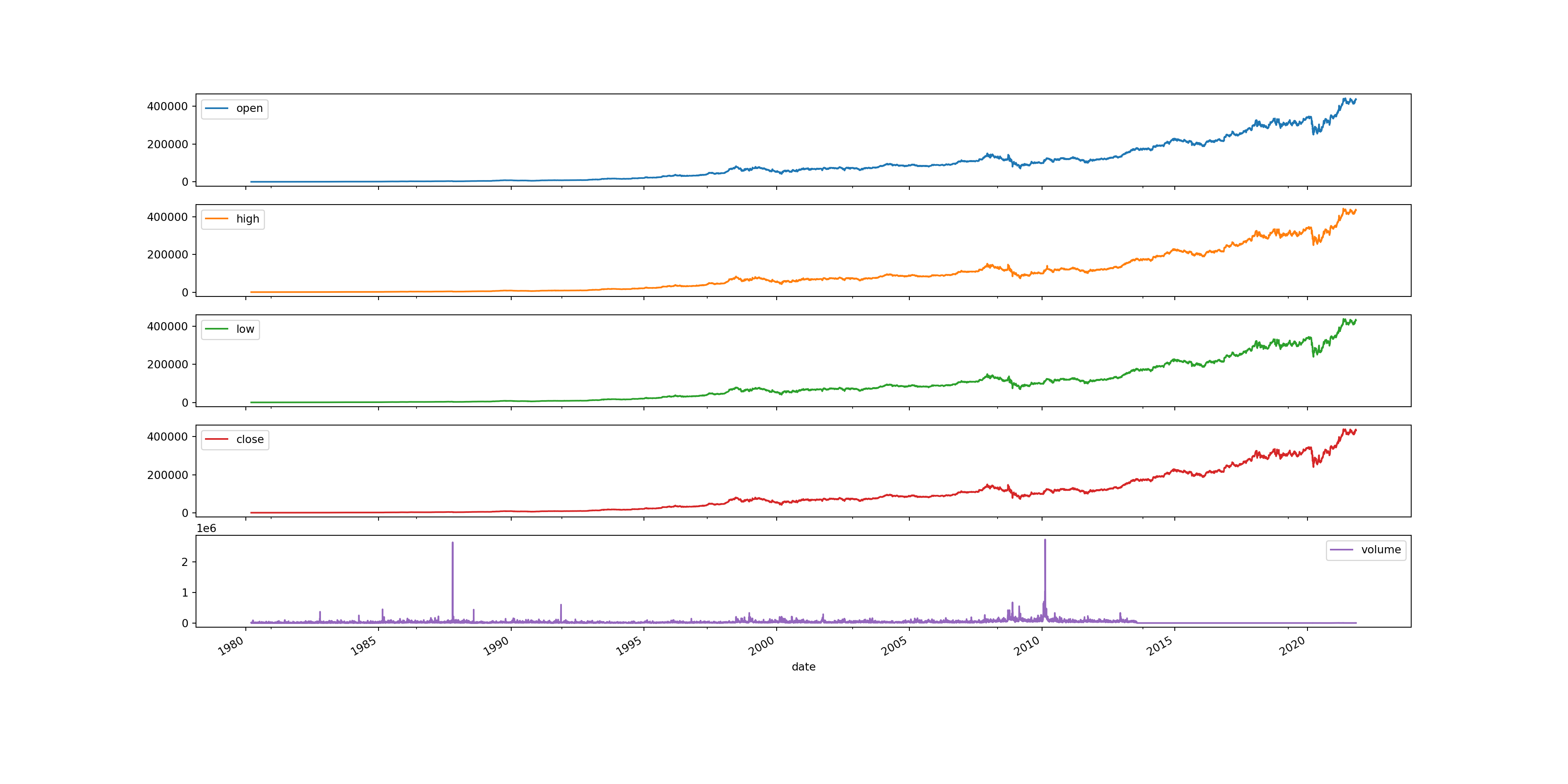
We can also check the correlation of different variables. Checking correlation helps to understand the relationship between different variables over time, identify leading/lagging indicators, and uncover potential causal links, which are important for forecasting and model building.
# view correlation of variables
brk.corr()
open high low close volume
open 1.000000 0.999952 0.999950 0.999912 -0.096983
high 0.999952 1.000000 0.999922 0.999954 -0.095437
low 0.999950 0.999922 1.000000 0.999952 -0.098510
close 0.999912 0.999954 0.999952 1.000000 -0.096585
volume -0.096983 -0.095437 -0.098510 -0.096585 1.000000Dot plot
A dot plot represents individual data points plotted along a timeline, allowing for the visualisation of trends, patterns, or changes over time. Each dot corresponds to an individual observation at a specific point in time, making it a straightforward method for displaying discrete measurements and detecting outliers or shifts within the time series data.
# creating a dot plot for the 'open' column
brk['open'].plot(style = 'k.', figsize = (20, 10))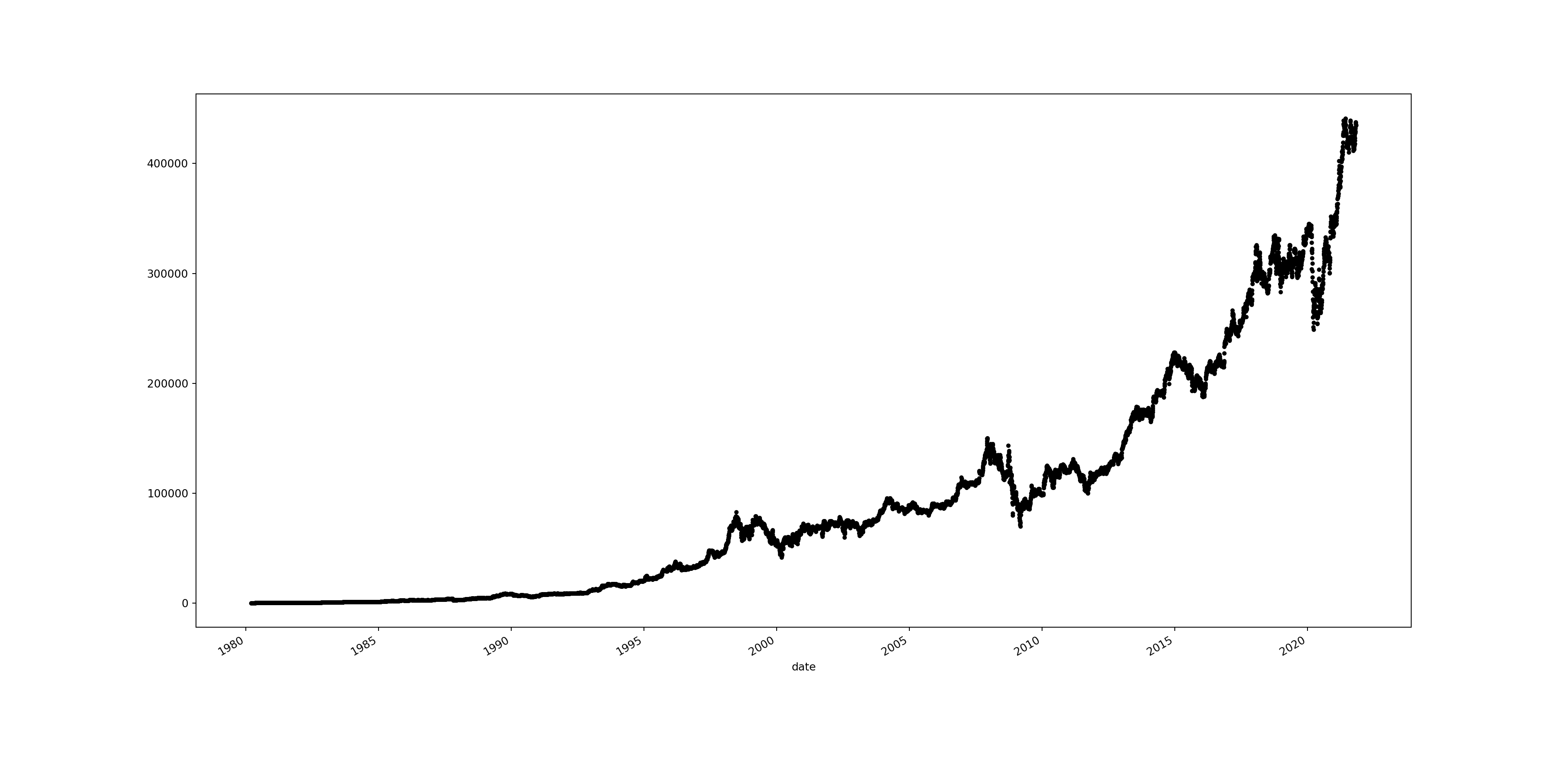
More style options: https://matplotlib.org/stable/users/prev_whats_new/dflt_style_changes.html
Group by years
# view the data by week
brk_week = brk.resample('1w').mean()
<string>:2: FutureWarning: 'w' is deprecated and will be removed in a future version, please use 'W' instead.# create an empty dataframe
years = pd.DataFrame()
# create groupby object containing annual data
groups = brk_week.groupby(pd.Grouper(freq = 'A'))<string>:3: FutureWarning: 'A' is deprecated and will be removed in a future version, please use 'YE' instead.
# extract name and group from the groupby object
for name, group in groups:
    # The year is extracted from the name
    year = name.year
    years[year] = group['open'].reset_index(drop=True)
years.head() 1980 1981 1982 ... 2019 2020 2021
0 290.0 423.75 560.0 ... 300178.750 339276.680 343964.0500
1 274.0 427.00 560.0 ... 295379.980 340219.200 346625.0000
2 262.5 425.00 548.0 ... 296125.500 342061.218 350187.4000
3 264.0 426.00 528.0 ... 302580.250 343636.500 352288.0625
4 254.0 430.00 506.0 ... 305244.998 336103.000 346884.9740
[5 rows x 42 columns]# create a plot for each year
years.plot(subplots = True, legend = True, figsize = (10, 30), sharex = True, sharey = True);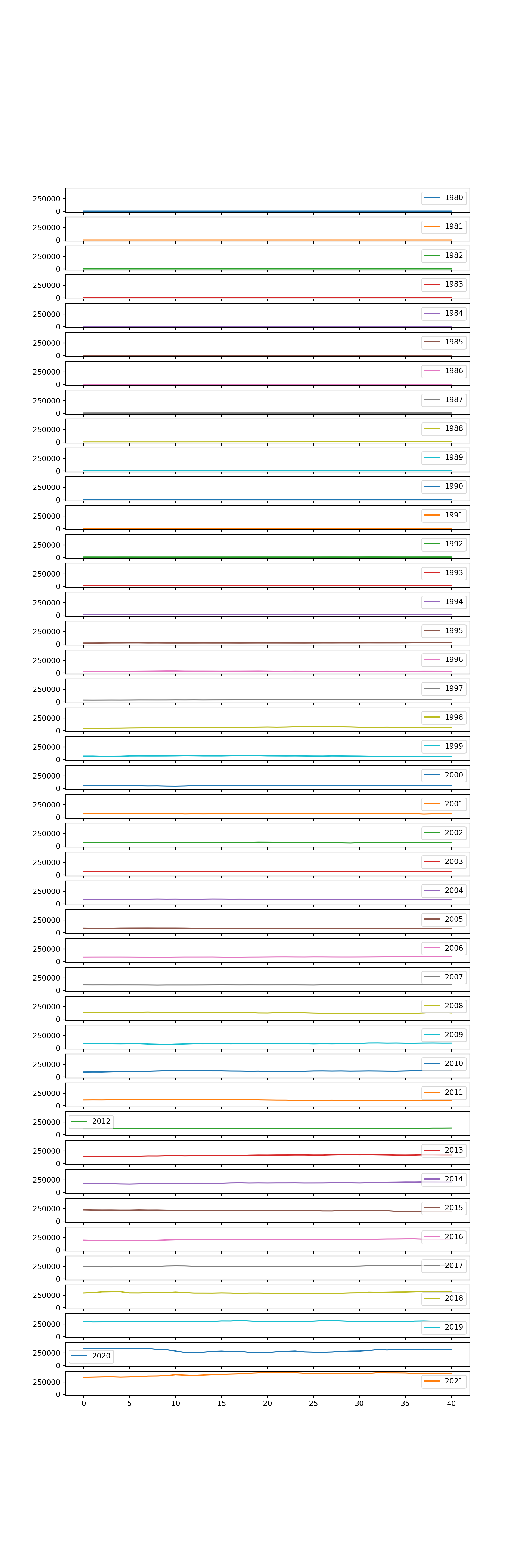
Box and Whisker plots
We can also create box and whisker plots in order to help us interpret the data. This can be very useful as it can help us to view outliers for a particular year, as well as see how spread the data is. This is particularly useful for identifying changes in data distribution over time.
years.boxplot(figsize = (20, 10))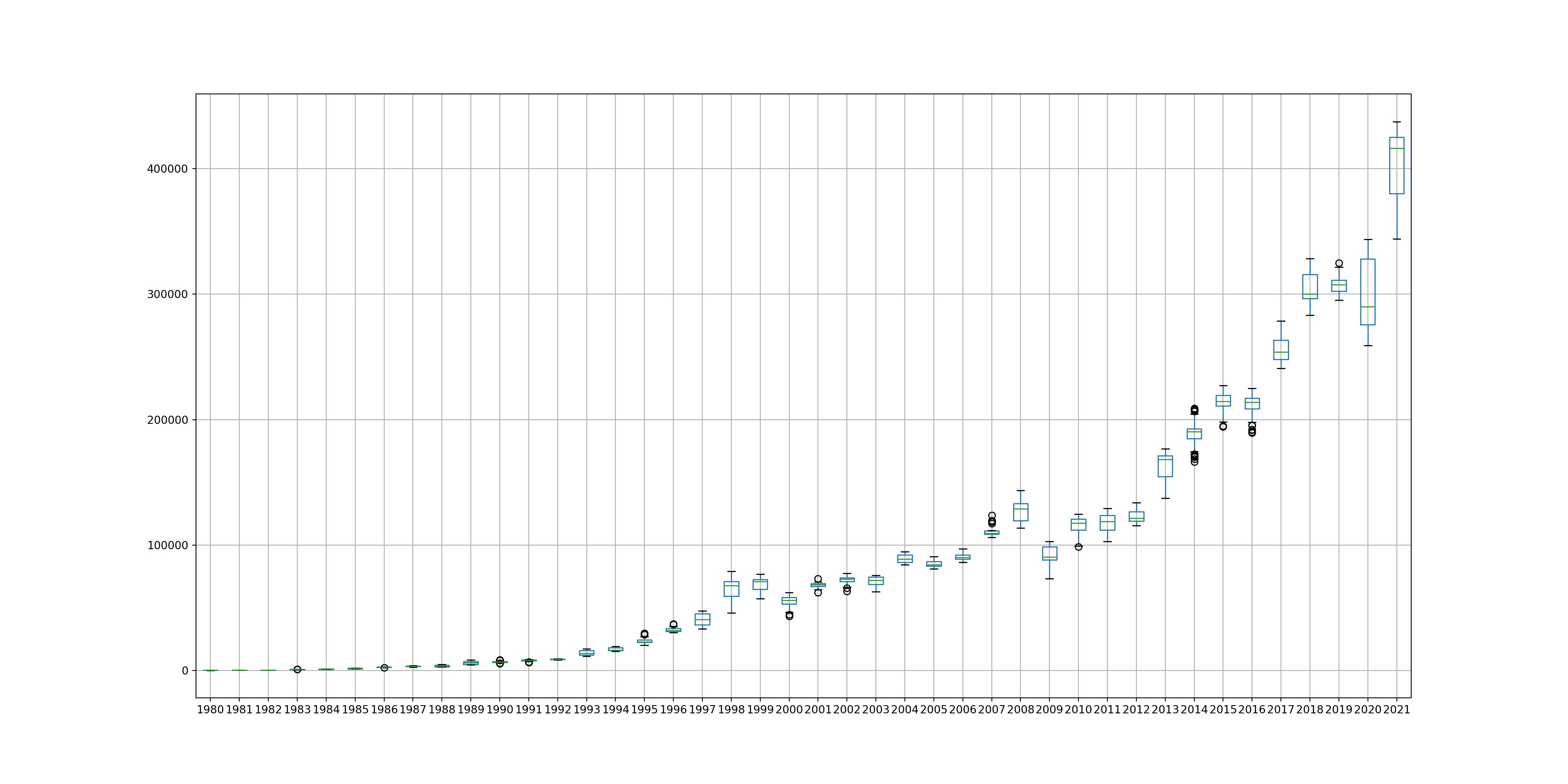
Heat Maps
Heatmaps are useful for analysing time series data because they provide a visual summary of complex information, allowing for quick identification of patterns, trends, and anomalies across time. By representing data values with colours, heatmaps make it easy to spot variations in intensity at a glance, such as periods of high or low activity.
# transpose the data
years_inverse = years.T
years_inverse.head() 0 1 2 3 ... 37 38 39 40
1980 290.00 274.0 262.5 264.0 ... 454.0 456.0 425.0 423.75
1981 423.75 427.0 425.0 426.0 ... 485.0 481.0 461.0 460.00
1982 560.00 560.0 548.0 528.0 ... 525.0 543.0 550.0 559.00
1983 772.00 776.0 787.0 775.0 ... 1153.0 1168.0 1232.0 1242.00
1984 1330.00 1300.0 1356.0 1348.0 ... 1291.0 1295.0 1301.0 1305.00
[5 rows x 41 columns]# create heatmap with seaborn
fig, ax = plt.subplots(figsize = (15, 10))
sns.heatmap(years_inverse)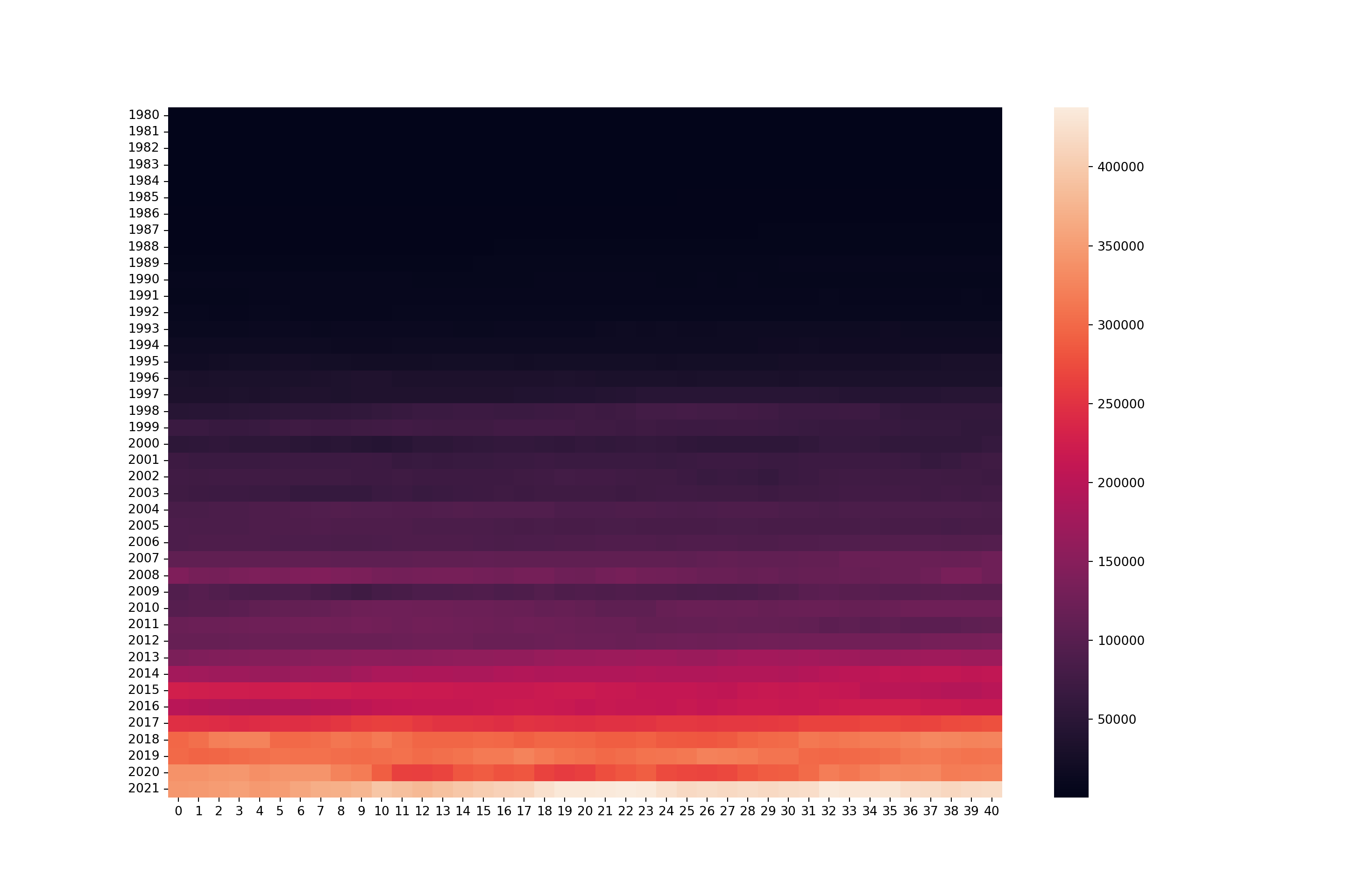
How would this be interpreted, taking into consideration what values the heatmap is showing?
Histogram and density plots
Histograms and density plots are valuable for analysing time series data as they provide insights into the distribution and density of data points over a specific period. These visualisations help identify patterns such as skewness, multimodality, and outliers, offering potential clues about underlying trends.
# create a histogram of the 'open' column
brk['open'].hist();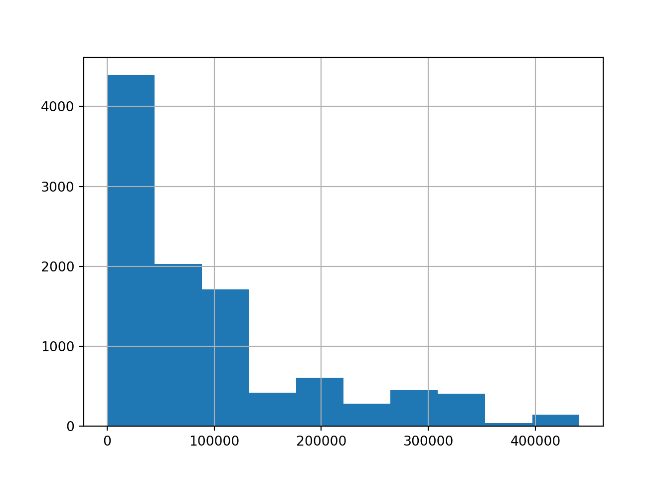
What does the histogram tell us about the data?
# create a kde plot of the data
brk['open'].plot(kind = 'kde');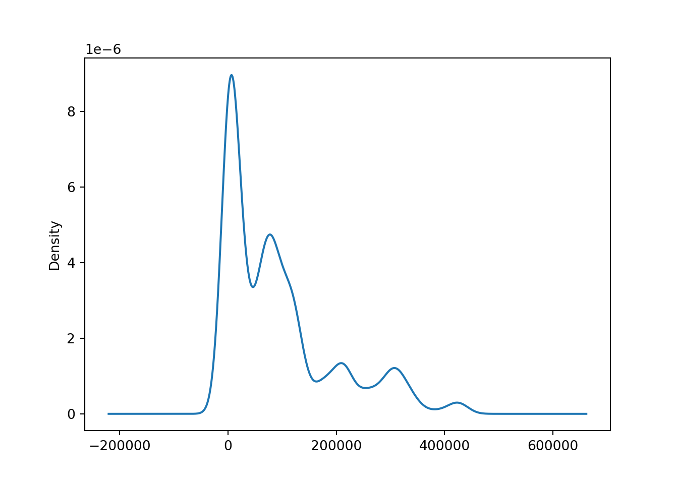
A kernel density estimate (KDE) plot is a method for visualizing the distribution of observations in a dataset, similar to a histogram. KDE represents the data using a continuous probability density curve in one or more dimensions
Scatter plot (lag plot)
A lag plot is a scatter plot used in time series analysis to help evaluate whether a data set or variable is random or has some time-dependent structure. It plots data points at time \(t\) on the x-axis and the data points at time \(t+n\) on the y-axis, where \(n\) is the lag amount.
If the points cluster along a diagonal line from the bottom-left to top-right, there is likely an autocorrelation indicating that the data is influenced by its prior values. Randomly scattered points suggest no such autocorrelation, indicating randomness in the data.
# lag plot for 'open' column
pd.plotting.lag_plot(brk['open'])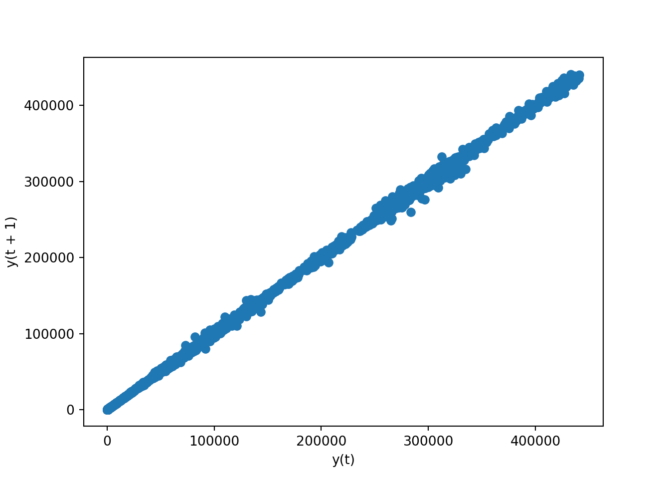
We can also use the lag parameter, which specifies the lag amount (the number of time periods to go back when comparing data points). With lag=7, the plot will compare each data point with the data point that is 7 periods before it. This is particularly useful in time series analysis to check for weekly seasonality – for instance, if you have daily data, lag=7 would help to see the correlation from one week to the next.
pd.plotting.lag_plot(brk['open'], lag = 7)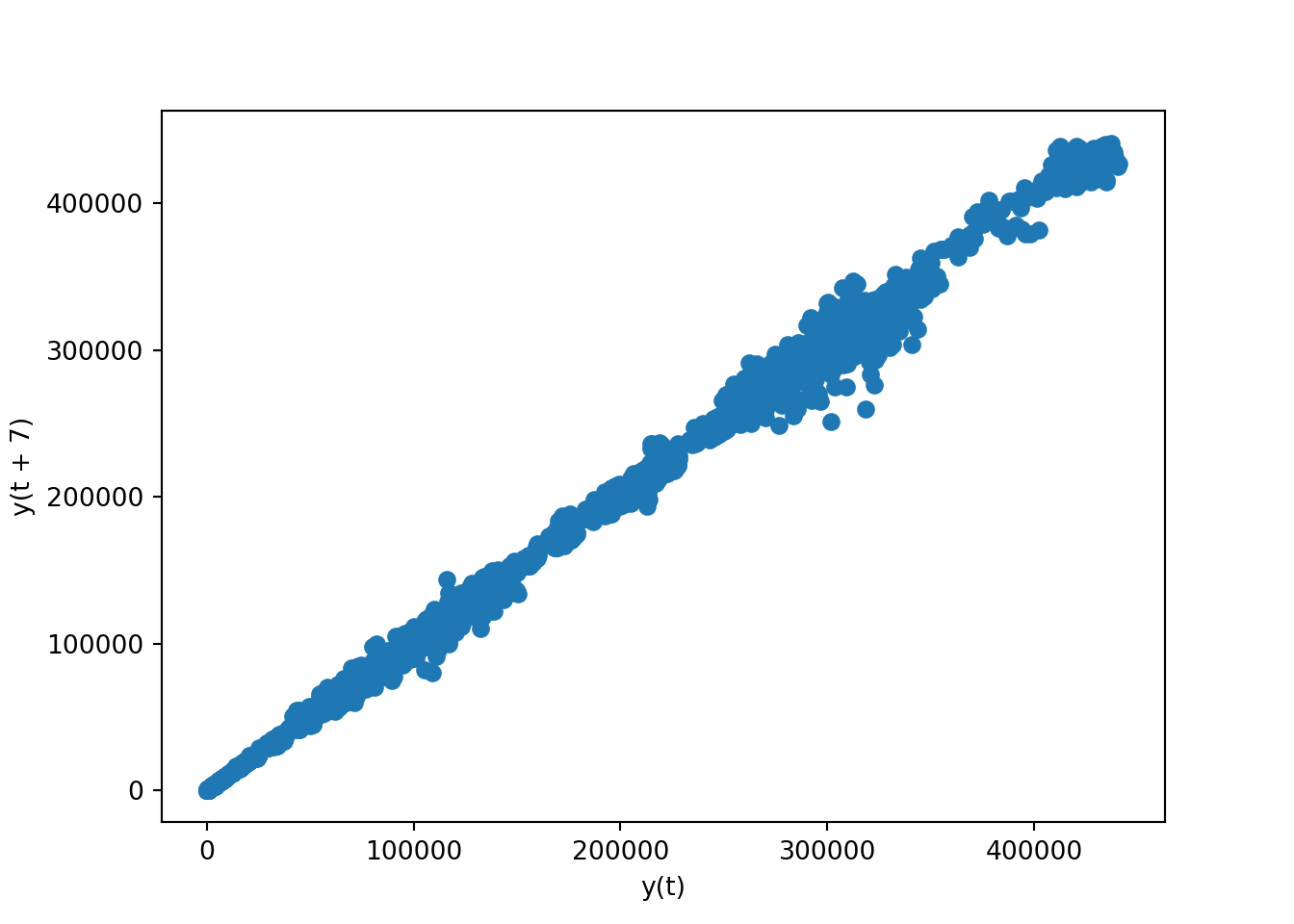
8.9 Decomposing time series data
There are three major components for any time series process: trend, seasonality, residual.
- Trend gives a sense of the long-term direction of the time series and can be either upward, downward or horizontal.
- Seasonality is repeated pattern over time. Example: Increasing of sales around Christmas each year.
- The residuals are the remaining or unexplained data points once we extract trend and seasonality.
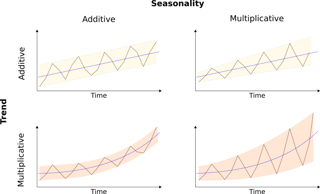
The decomposition of a time series is the process of extracting these three components. The modelling of the decomposed components can be either additive or multiplicative.
Based on the additive model we can reconstruct the original time series by adding all three components.
y = Trend + Seasonality + Residual
The additive model should be applied when the seasonal variations do not change over time.
Based on the multiplicative model we can reconstruct the time series data by multiplying the 3 components.
y = Trend x Seasonality x Residual
# plot the open column
brk_week['open'].plot()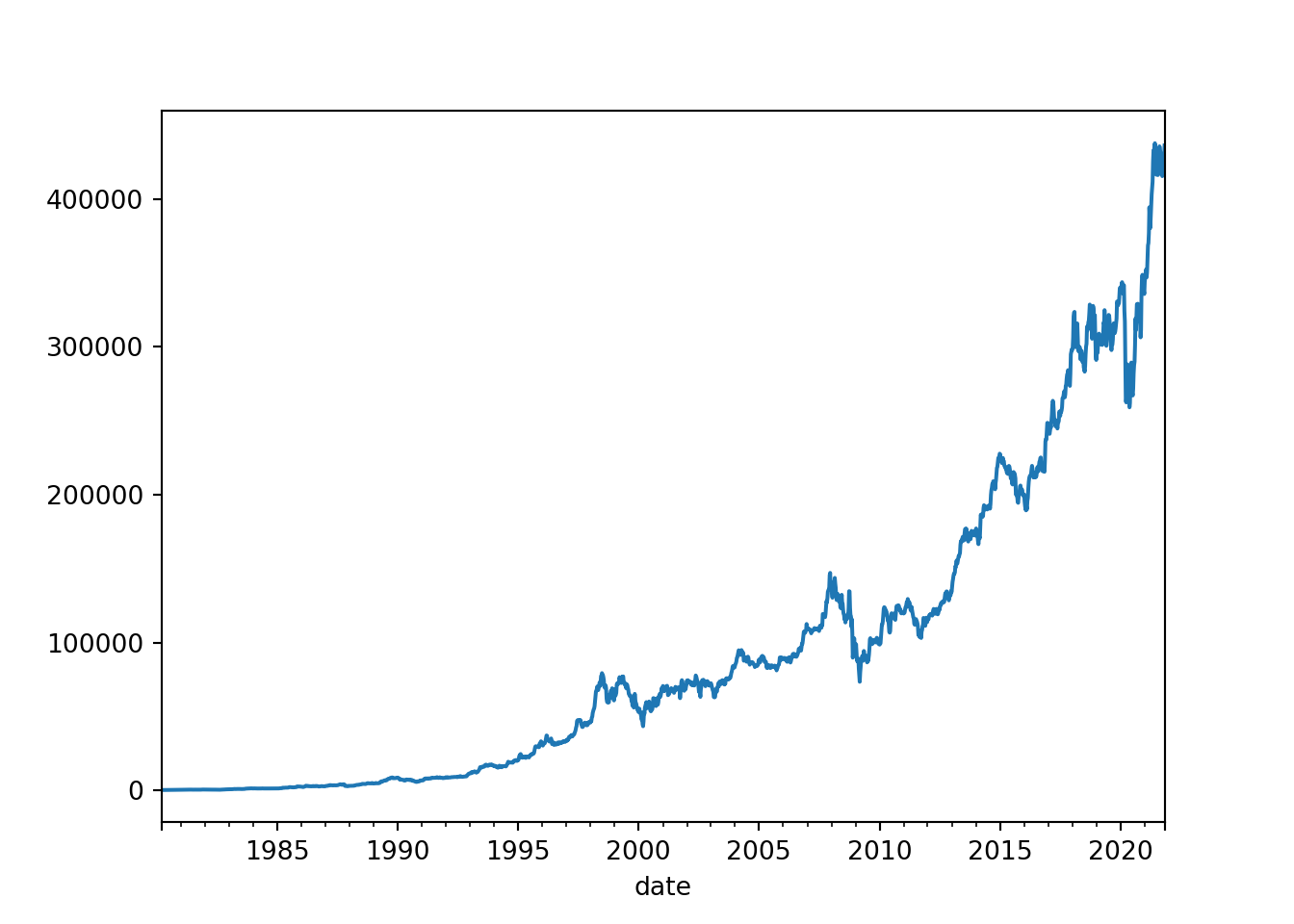
# import packages
from statsmodels.tsa.seasonal import seasonal_decompose, STL
Link to seasonal decomposition documentation:
brk_week_decomposed = seasonal_decompose(brk_week['open'], model = 'multiplicative') # model is optionalWhen you don’t specify the model parameter, seasonal_decompose defaults to using the “additive” model because many time series with a seasonal component can be adequately modeled with additive effects, especially when the seasonal fluctuations do not vary much in scale over time.
plt.rcParams['figure.figsize'] = (10,5)
brk_week_decomposed.plot()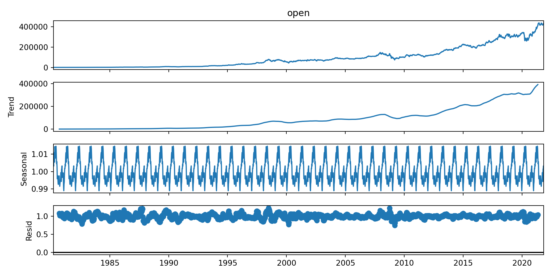
- The first chart - The original observed data
- The trend shows an upward direction - positive(also can be negative or constant)
- The seasonal component shows the repeating pattern of highs and lows.
- The residual component shows the random variation in the data, and is what is left over after fitting a model.
8.10 Checking for Stationarity
Example - bicycle data
# read in data
bicycles = pd.read_csv("data/bicycle_rent.csv")

# convert start time column to datetime format
bicycles['starttime'] = pd.to_datetime(bicycles['starttime'], format ='%Y-%m-%d %H:%M:%S')

# convert start time column to index
bicycles_date = bicycles.set_index('starttime')

# resample data to months
bicycles_date['count'] = 1 # create a count column to tally eventd
bicycles_months = bicycles_date.resample('1m').count()
<string>:1: FutureWarning: 'm' is deprecated and will be removed in a future version, please use 'ME' instead.bicycles_months.info()<class 'pandas.core.frame.DataFrame'>
DatetimeIndex: 33 entries, 2014-01-31 to 2016-09-30
Freq: ME
Data columns (total 4 columns):
# Column Non-Null Count Dtype
--- ------ -------------- -----
0 stoptime 33 non-null int64
1 tripduration 33 non-null int64
2 temperature 33 non-null int64
3 count 33 non-null int64
dtypes: int64(4)
memory usage: 1.3 KB# create a series consisting of count column
series = bicycles_months[['count']]# plot the series
series.plot()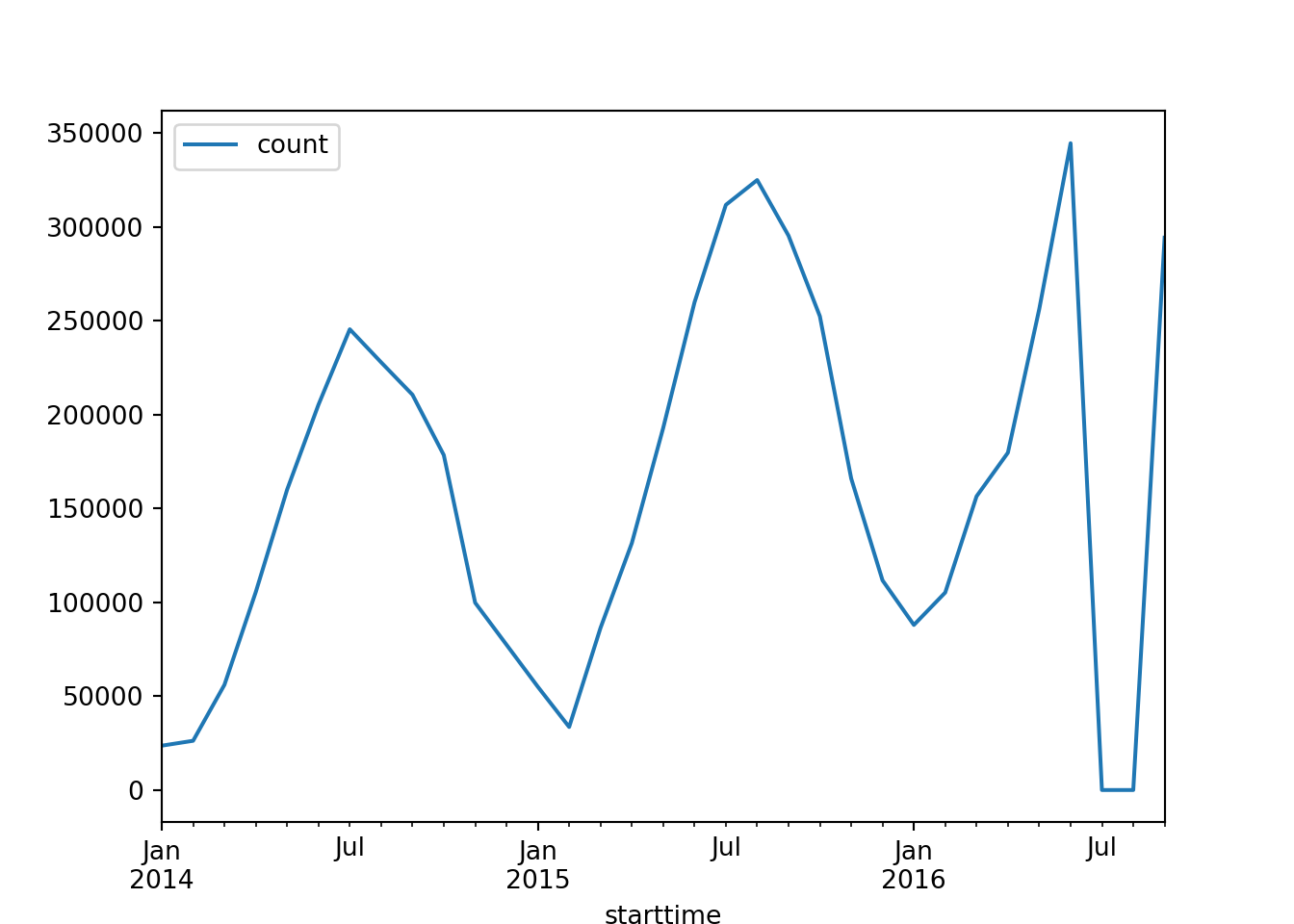
Many forecasting techniques assume stationarity. That’s why it is crucial to understand if the data we are working with is stationary or non-stationary.
A stationary time series doesn’t have a trend or seasonality. Thus the data don’t have patterns or specific statistical properties that vary over time. This kind of data makes the process easier to model and predict.
Non-stationary data contains patterns that might vary over time, making the modelling process more complex due to the dynamic nature of the data.
8.10.1 The Augmented Dickey-Fuller Test
The Augmented Dickey-Fuller (ADF) test is used to check if a series is stationary.
- Null Hypothesis \((H_0)\): The series is non-stationary.
- Alternative Hypothesis \((H_1)\): The series is stationary.
How Does the ADF Test Work?
The test incorporates lagged (past) values of the time series to account for any autocorrelation. After running the test, we compare the test statistic to critical values at various confidence levels. If the test statistic is less than the critical value, we reject the null hypothesis, suggesting the series does not have a unit root and is likely stationary.
Why is the ADF Test Important?
Understanding whether a time series is stationary is essential before applying most forecasting models, as these models assume stationarity.
https://www.statsmodels.org/dev/generated/statsmodels.tsa.stattools.adfuller.html
from statsmodels.tsa.stattools import adfulleradfuller(series)(-1.732429016531073, 0.4144862524209757, 8, 24, {'1%': -3.7377092158564813, '5%': -2.9922162731481485, '10%': -2.635746736111111}, 555.2839223446316)
# pvalue of 1 > 0.05 ===> The null hypothesis cannot be rejected.
# Hence data is non-stationary (it has relation with time)
The result is a tuple with the following information:
ADF Statistic: This is the value of the test statistic. The more negative this statistic, the stronger the rejection of the hypothesis that there is a unit root at some level of confidence. In other words, more negative values suggest the series is stationary.
p-value: This represents the probability of observing the test results under the null hypothesis. In this case, the p-value is relatively high, suggesting that there is not enough evidence to reject the null hypothesis of the presence of a unit root, meaning the time series might be non-stationary.
Critical values: These values represent the test statistic values needed to reject the null hypothesis of a unit root presence at the 1%, 5%, and 10% levels of significance, respectively. Our ADF statistic is not more negative than any of these, suggesting we cannot reject the null hypothesis for any usual level of significance.
Because the bike data is not stationary, we need to perform some transformations.
8.11 Detrending
Detrending refers to the process of removing trends from a time series. Trends represent long-term movements in data, which can be linear (steady increase or decrease over time) or non-linear (seasonal or cyclical patterns). The practice of detrending is pivotal for several reasons:
Achieving Stationarity: Time series analysis and forecasting models often presume stationarity, where the statistical properties (mean, variance) of the series are constant over time. Detrending is a critical step towards converting a non-stationary series into a stationary one by eliminating the underlying trends.
Understanding Data Better: By removing the trend, it becomes easier to isolate and analyze the data’s fluctuations or noise not explained by the trend. This can uncover insights into the data’s underlying mechanisms or reveal hidden patterns.
Enhancing Forecasting Accuracy: Forecasting models developed on detrended data can be more accurate, as they focus on predicting the stationary components of the series (like seasonal variations) without being influenced by long-term trends.
Comparing Different Time Series: Detrending allows for the comparison of different time series data on an equal footing by removing their underlying trends, facilitating a more straightforward analysis and understanding.
Detrending is an important preprocessing step in time series analysis, enabling more precise analysis, modelling, and forecasting by focusing on the intrinsic properties of the data, independent of any trend.
8.12 Differentiating
# creating a dataframe for the series - we want to add lag to the data and will need a new column for this
series_df = pd.DataFrame(series)

# add shifted data to new column
series_df['shifted_1lag'] = series_df.shift(1)

series_df.head()
count shifted_1lag
starttime
2014-01-31 23617 NaN
2014-02-28 26221 23617.0
2014-03-31 56020 26221.0
2014-04-30 105428 56020.0
2014-05-31 159957 105428.0Next, we need to perform differentiation between the orginal series and the lagged series. This will then give us the difference between the two ‘count’ values.
# create new column for the difference
series_df['series_diff'] = series_df['count'] - series_df['shifted_1lag']
series_df.head()
count shifted_1lag series_diff
starttime
2014-01-31 23617 NaN NaN
2014-02-28 26221 23617.0 2604.0
2014-03-31 56020 26221.0 29799.0
2014-04-30 105428 56020.0 49408.0
2014-05-31 159957 105428.0 54529.0We now perform the ADF test again, this time on the series_diff column.
pvalue = adfuller(series_df['series_diff'][1:])[1] # from second row onwards
pvalue0.8341986459358672if pvalue > 0.05:
print('data is non-stationary')
else:
print('data is stationary')data is non-stationary# plot the series difference data
series_df['series_diff'].plot()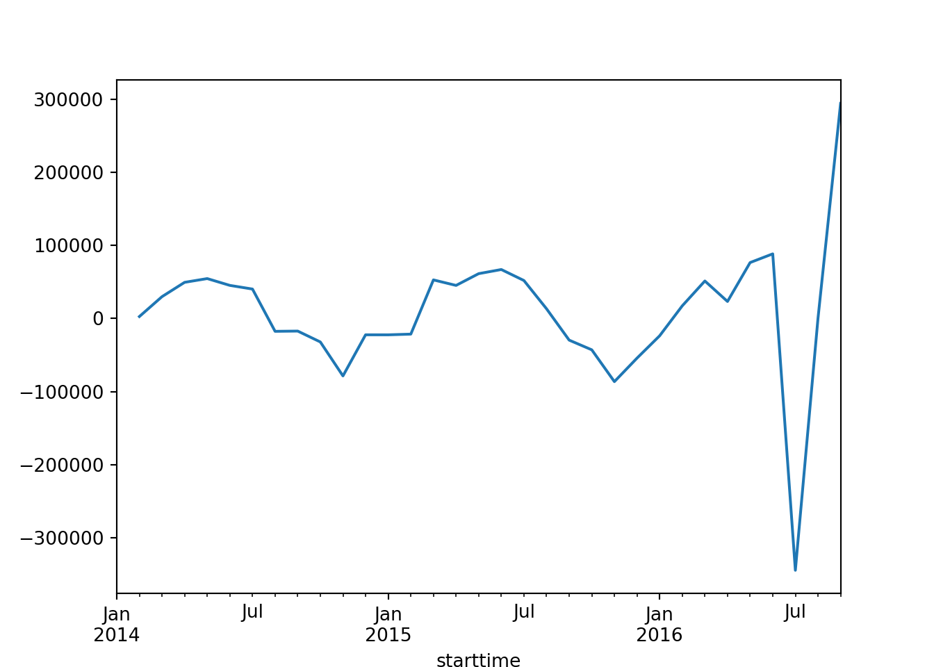
As the data is not stationary, we need to perform differencing again.
# Add second differencing
series_df['series_diff_2'] = series_df['series_diff'].diff()

# perform the ADF test on the second difference
pvalue_second_diff = adfuller(series_df['series_diff_2'].dropna())[1]  # from the second row onwards due to differencing

print(pvalue_second_diff)2.1744798473897922e-06if pvalue_second_diff > 0.05:
print('Data is still non-stationary after second differencing.')
else:
print('Data is stationary after second differencing.')Data is stationary after second differencing.# plot the series difference data
series_df['series_diff_2'].plot()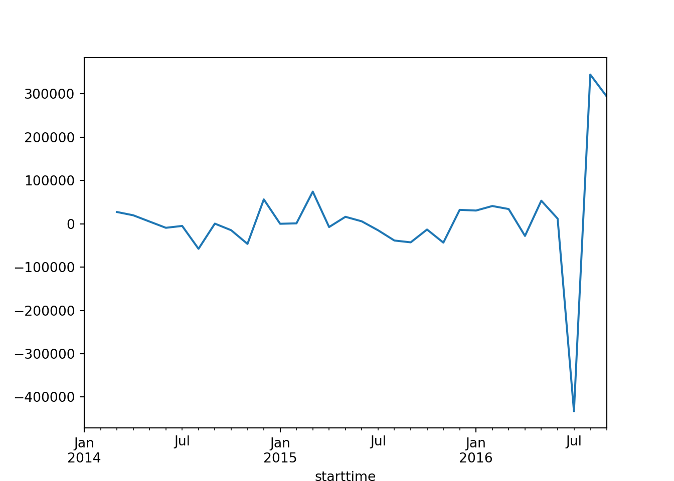
8.13 White noise
Example
First, we will generate a series which will contain 1000 data points. It is drawn from a normal distribution with mean 0 and standard deviation of 1, meaning the numbers are very likely (99.9999%) to be between -4 and 4.
# generate data
import random

random.seed(1)
series = []
for i in range(1000):
    n = random.gauss(0, 1)
    series.append(n)
# view information about the series
series = pd.Series(series)
series.describe()count 1000.000000
mean -0.013222
std 1.003685
min -2.961214
25% -0.684192
50% -0.010934
75% 0.703915
max 2.737260
dtype: float64What do we notice about the mean? Does this mean we have white noise?
# plot the data
series.plot()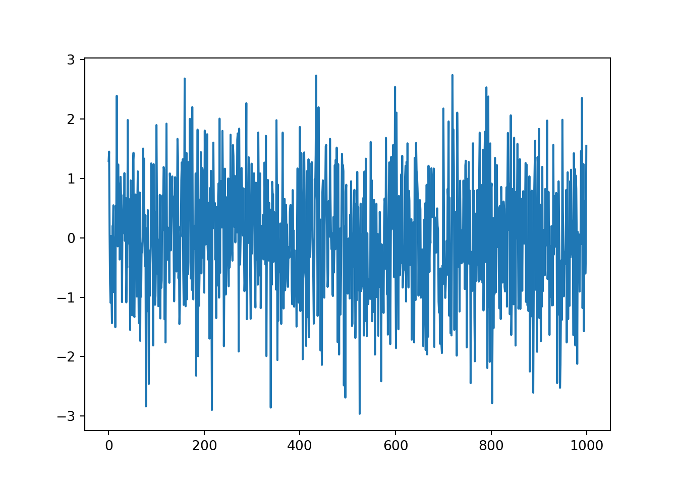
It’s very hard to find patterns in the data at the moment.
We can also view it as a histogram.
# view series as a histogram
series.hist()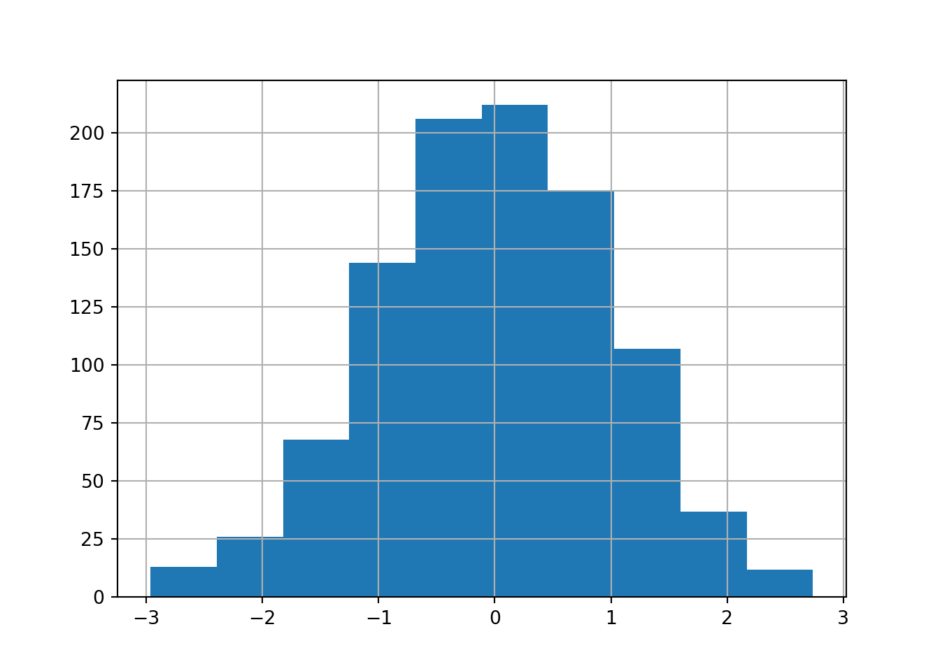
# lag the data with default 1
pd.plotting.lag_plot(series)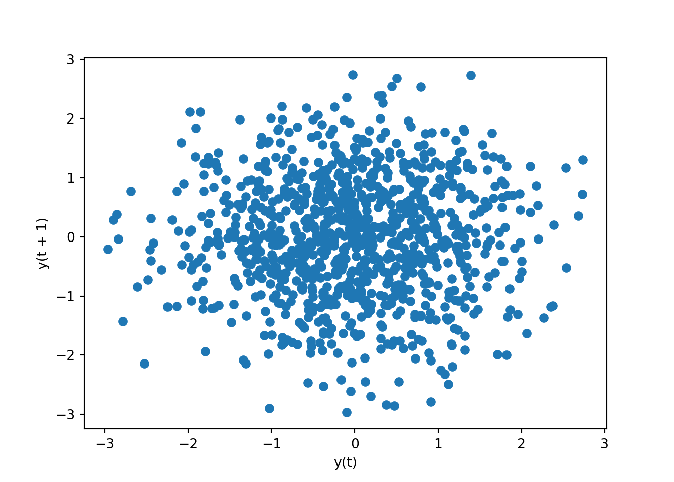
There are no patterns, which means there is no autocorrelation between a specific time and its lag.
We can import a new package from pandas, called autocorrelation_plot, which shows whether the elements of a time series are correlated with each other. Lag is on the x axis and Autocorrelation is on the y axis (correlation between the original series and the lagged data.
from pandas.plotting import autocorrelation_plot

# plot the series
autocorrelation_plot(series)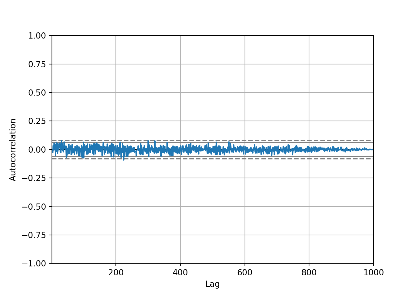
To interpret the autocorrelation plot:
Autocorrelation represents the degree of similarity between a given time series and a lagged version of itself over successive time intervals.
Autocorrelation measures the relationship between a variable’s current value and its past values.
An autocorrelation of +1 represents a perfect positive correlation, while an autocorrelation of -1 represents a perfect negative correlation.
All of the values for autocorrelation are very low (around 0). The grey lines, which are the boundaries of confidence, shouldn’t have any blue points that cross it, which means there is no significant correlation in this dataset.
8.14 Random walk
Example
The below function will randomly add one or minus one value. This is to simulate a step in either the positive or negative direction.
random.seed(2021)
random_walk_values = []
random_walk_values.append(-1 if random.random() < 0.5 else 1)

for i in range(1, 1000):
    movement = -1 if random.random() < 0.5 else 1
    value = random_walk_values[i-1] + movement
    random_walk_values.append(value)
# plot the random walk values
plt.plot(random_walk_values)
# autocorrelation plot of random walk values
autocorrelation_plot(random_walk_values)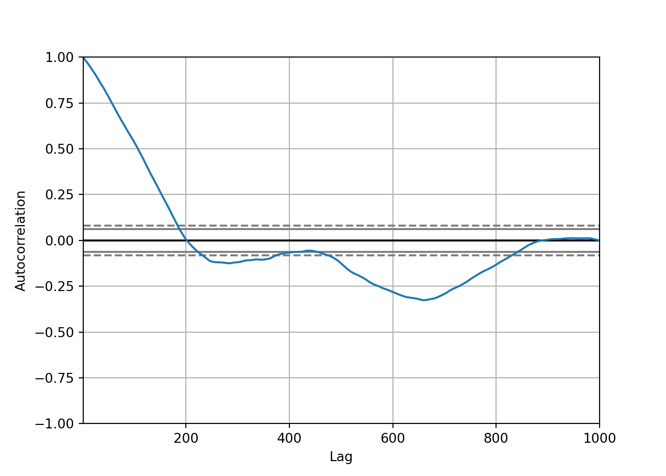
Interpretation:
The autocorrelation starts off strong at lag 0 (as it always does) and decreases sharply as the lag increases. This is typical for many time series, where the immediate past is often more informative than the more distant past.
There are points where the autocorrelation dips below the lower confidence bound, suggesting significant negative autocorrelation at certain lags. This might indicate a cyclical pattern where the values oscillate in a fixed pattern over time.
Beyond a certain point, the autocorrelation seems to hover around zero, not crossing the significance bounds, implying no significant correlation at those lags.
We can now check the stationarity of this data using the ADF test.
# test stationarity of random walk values
adfuller(random_walk_values)
(-1.326616691277989, 0.6169088978451089, 1, 998, {'1%': -3.4369193380671, '5%': -2.864440383452517, '10%': -2.56831430323573}, 2774.6156168271864)We need to differentiate the data to make it stationary.
# differentiate the data
diff = []
for i in range(1, len(random_walk_values)):
    value = random_walk_values[i] - random_walk_values[i - 1]
    diff.append(value)
# plot the values
plt.plot(diff)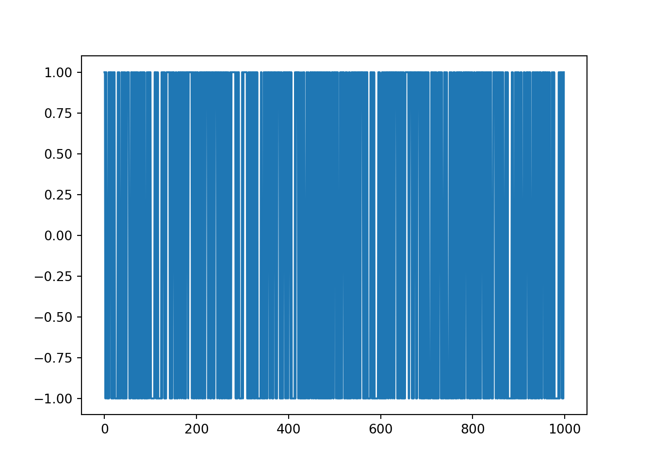
The output of this plot means that it is essentially white noise and there is no structure to the data. It is unable to be used for forecasting.
# autocorrelation plot of differentiated values
autocorrelation_plot(diff)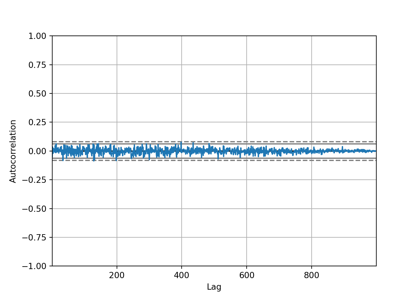
The autocorrelation is very close to 0 so we would have no information to give to our model.
8.15 Train-test split
First, we need to split the data into training data and test data, using the count column. It’s important to note we are using the original count column, not the differentiated column that we looked at in the last notebook. This is because the ARIMA model has a component which will automatically differentiate the data for us. When the ARIMA model gives you the results back, it will convert it to the original data, but if the differentiation is performed outside of the ARIMA, you have the difference between two months which is harder to interpret when forecasting.
bicycles_months.head() stoptime tripduration temperature count
starttime
2014-01-31 23617 23617 23617 23617
2014-02-28 26221 26221 26221 26221
2014-03-31 56020 56020 56020 56020
2014-04-30 105428 105428 105428 105428
2014-05-31 159957 159957 159957 159957series = series_df['count']Our training data will be the data before and including 31st December 2016. The test data will be everything after that.
Note: Train-test split is different to what we have previously performed, where the data was split randomly. Time series data should be split based on time to maintain the integrity of the temporal order. Typically, you would allocate the earlier portion of the data for training and the later portion for testing.
# defining train and test data
train = series[:'2015-12-31']
test = series['2015-10-31':]
8.16 AR (Autoregressive) Model
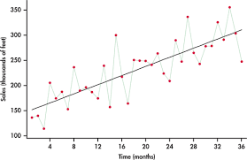
The image below shows data about the number of passengers on a certain bus route in a village. The original series, t, starts in September, but if we move backward to t-1, the series starts in August. If we move backward two units, the series starts with July, and so on.
The AR model will try to understand which predictor will be the most important - e.g, does t-1 predict t better than t-2?
This is called an AR(4) model as it is using the four previous time points to forecast the current time point, t. More generally it is called an AR(p) model.
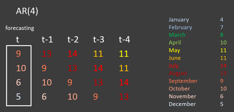
The AR model formula:
Where \(\alpha\) is the constant (series mean),
\(\beta_n\) are the coefficients,
\(Y_{t-n}\) are the predictors,
\(\epsilon\) is the error term (white noise)
8.16.1 AR(1)
from statsmodels.tsa.arima.model import ARIMAThe ARIMA model, short for Autoregressive Integrated Moving Average, is a forecasting algorithm that is used to predict future points in a time series. It is composed of three parts:
AR (Autoregressive): The model uses the dependent relationship between an observation and some number of lagged observations (
p).I (Integrated): The model employs differencing of observations (the number of differences needed to make the series stationary, denoted by
d).MA (Moving Average): The model incorporates the dependency between an observation and a residual error from a moving average model applied to lagged observations (
q).
The model is typically denoted as ARIMA(p, d, q) where p is the order of the autoregressive terms, d is the degree of differencing, and q is the order of the moving average process.
# create the model on the train data
model = ARIMA(train, order = (1,0,0)) # 1 - number of lags
results = model.fit()

results.summary()| Dep. Variable: | count | No. Observations: | 24 |
| Model: | ARIMA(1, 0, 0) | Log Likelihood | -291.720 |
| Date: | Mon, 22 Apr 2024 | AIC | 589.441 |
| Time: | 17:09:23 | BIC | 592.975 |
| Sample: | 01-31-2014 | HQIC | 590.378 |
| - 12-31-2015 | |||
| Covariance Type: | opg |
| coef | std err | z | P>|z| | [0.025 | 0.975] | |
| const | 1.598e+05 | 5.02e+04 | 3.183 | 0.001 | 6.14e+04 | 2.58e+05 |
| ar.L1 | 0.8825 | 0.112 | 7.909 | 0.000 | 0.664 | 1.101 |
| sigma2 | 1.873e+09 | 0.643 | 2.91e+09 | 0.000 | 1.87e+09 | 1.87e+09 |
| Ljung-Box (L1) (Q): | 12.40 | Jarque-Bera (JB): | 1.50 |
| Prob(Q): | 0.00 | Prob(JB): | 0.47 |
| Heteroskedasticity (H): | 1.84 | Skew: | -0.15 |
| Prob(H) (two-sided): | 0.41 | Kurtosis: | 1.81 |
Warnings:
[1] Covariance matrix calculated using the outer product of gradients (complex-step).
[2] Covariance matrix is singular or near-singular, with condition number 4.54e+25. Standard errors may be unstable.
Main points of interest from the summary of results:
There are 36 observations
AIC/BIC/HQIC - information criteria used to compare models with different numbers of parameters. They take into account the goodness of fit and the complexity of the model (penalizing for more parameters). A lower value indicates a better model according to that criterion
Coefficient - the constant is usually the mean of the series.
ar.L1 - this means we used one lag, and the coefficient (\(\beta\)) is 0.88
sigma2 - the error term.
P>|z| - The p-value associated with the z-test for each coefficient, testing the null hypothesis that the coefficient is zero against the alternative that it is not zero.
Ljung-Box (Q) - A test statistic for the null hypothesis that the model does not show lack of fit, i.e., the residuals are independently distributed. A small p-value (Prob(Q)) indicates that the residuals are uncorrelated.(white noise)
Jarque-Bera (JB) - A test statistic for the null hypothesis that the residuals are normally distributed. The p-value (Prob(JB)) indicates whether the residuals depart from normality.
Heteroskedasticity (H) - a test statistic for the null hypothesis that the residuals have constant variance (are homoskedastic). A high p-value (Prob(H)) indicates that you cannot reject the null of homoskedasticity.
train.mean()159841.33333333334We can also get some predictions by using get_prediction, specifying the time period that we want to predict.
# get prediction
forecast = results.get_prediction(start = '2016-09-30', end = '2017-08-31')
confidence_intervals = forecast.conf_int()
confidence_intervals lower count upper count
2016-09-30 -26377.582236 314771.380240
2016-10-31 -26747.095132 318817.819387
2016-11-30 -26824.853416 322140.408188
2016-12-31 -26705.767775 324884.835265
2017-01-31 -26457.795300 327163.868451
2017-02-28 -26129.625185 329065.741726
2017-03-31 -25756.012865 330660.108189
2017-04-30 -25361.562085 332002.368231
2017-05-31 -24963.450032 333136.876604
2017-06-30 -24573.414499 334099.354879
2017-07-31 -24199.215410 334918.728295
2017-08-31 -23845.716039 335618.538190Confidence intervals may be useful to us, because they represent the pessimistic and optimistic margins.
Pessimistic margins - the lower values the model has given us. They consider the worst possibilities but often overestimate the worst-case scenario
Optimistic margins - the upper values the model has given us. This would be the best case scenario.
The mean will be the average of these two values.
# mean of the forecasting values
forecast_mean = forecast.predicted_meanforecast_mean2016-09-30 144196.899002
2016-10-31 146035.362128
2016-11-30 147657.777386
2016-12-31 149089.533745
2017-01-31 150353.036575
2017-02-28 151468.058271
2017-03-31 152452.047662
2017-04-30 153320.403073
2017-05-31 154086.713286
2017-06-30 154762.970190
2017-07-31 155359.756443
2017-08-31 155886.411076
Freq: ME, Name: predicted_mean, dtype: float64We can now plot the forecasted values.
plt.plot(series) # the original data
plt.plot(results.fittedvalues, # estimated values from the model
         color = 'orange',
         label = 'forecast')
plt.plot(forecast_mean, color = 'red') # forecast mean
plt.fill_between(forecast_mean.index, # display the lower and upper count
                confidence_intervals['lower count'],
                confidence_intervals['upper count'],
                color = 'pink',
                alpha = 0.5)
plt.xticks(rotation = 45);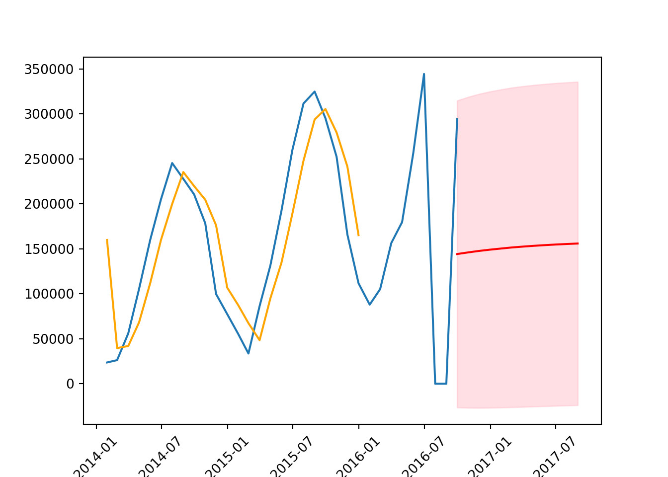
The margins are very large. This means the model is very uncertain and often the further into the future you go, the wider the margin will be.
We can also comput the mean squared error, to evaluate the accuracy of a model’s prediction. The “squared” aspect emphasises larger errors over smaller ones, meaning it punishes large errors more severely than small ones, which can be particularly useful in identifying models that might occasionally be very inaccurate.
Lower MSE: Indicates a model that predicts the observed data with higher accuracy. A lower MSE is generally preferable, as it means the model’s predictions are closer to the actual values.
Higher MSE: Indicates that the model’s predictions deviate more significantly from the actual observed values. A high MSE suggests the model may not be capturing the underlying pattern of the series effectively.
from sklearn.metrics import mean_squared_error

mean_squared_error(test, forecast_mean, squared = False) # returns root mean squared error (RMSE)
105656.8487371978
C:\Users\GEORGI~1\AppData\Local\Programs\Python\PYTHON~1\Lib\site-packages\sklearn\metrics\_regression.py:483: FutureWarning: 'squared' is deprecated in version 1.4 and will be removed in 1.6. To calculate the root mean squared error, use the function'root_mean_squared_error'.
warnings.warn(In the context of bike trips, it means that, on average, the model’s predictions were about 105,656 trips different from the actual numbers.
Now we can try an AR model with two lags rather than one, to see if this will improve the results.
8.16.2 AR(2)
# create model
model = ARIMA(train, order = (2,0,0))
results = model.fit()

# summarise results
results.summary()| Dep. Variable: | count | No. Observations: | 24 |
| Model: | ARIMA(2, 0, 0) | Log Likelihood | -275.985 |
| Date: | Mon, 22 Apr 2024 | AIC | 559.970 |
| Time: | 17:09:29 | BIC | 564.683 |
| Sample: | 01-31-2014 | HQIC | 561.220 |
| - 12-31-2015 | |||
| Covariance Type: | opg |
| coef | std err | z | P>|z| | [0.025 | 0.975] | |
| const | 1.598e+05 | 2.08e+04 | 7.691 | 0.000 | 1.19e+05 | 2.01e+05 |
| ar.L1 | 1.6357 | 0.102 | 16.058 | 0.000 | 1.436 | 1.835 |
| ar.L2 | -0.8695 | 0.100 | -8.701 | 0.000 | -1.065 | -0.674 |
| sigma2 | 4.686e+08 | 0.684 | 6.85e+08 | 0.000 | 4.69e+08 | 4.69e+08 |
| Ljung-Box (L1) (Q): | 4.21 | Jarque-Bera (JB): | 0.49 |
| Prob(Q): | 0.04 | Prob(JB): | 0.78 |
| Heteroskedasticity (H): | 1.06 | Skew: | -0.13 |
| Prob(H) (two-sided): | 0.94 | Kurtosis: | 2.35 |
Warnings:
[1] Covariance matrix calculated using the outer product of gradients (complex-step).
[2] Covariance matrix is singular or near-singular, with condition number 3.89e+24. Standard errors may be unstable.
# get predictions and confidence intervals
forecast = results.get_prediction(start = '2017-01-31', end = '2017-12-31')
forecast_mean = forecast.predicted_mean
confidence_intervals = forecast.conf_int()
# plot the data
plt.plot(series)
plt.plot(results.fittedvalues,
color = 'orange',
label = 'forecast')
plt.plot(forecast_mean, color = 'red')
plt.fill_between(forecast_mean.index,
confidence_intervals['lower count'],
confidence_intervals['upper count'],
color = 'pink',
alpha = 0.5)
plt.xticks(rotation = 45);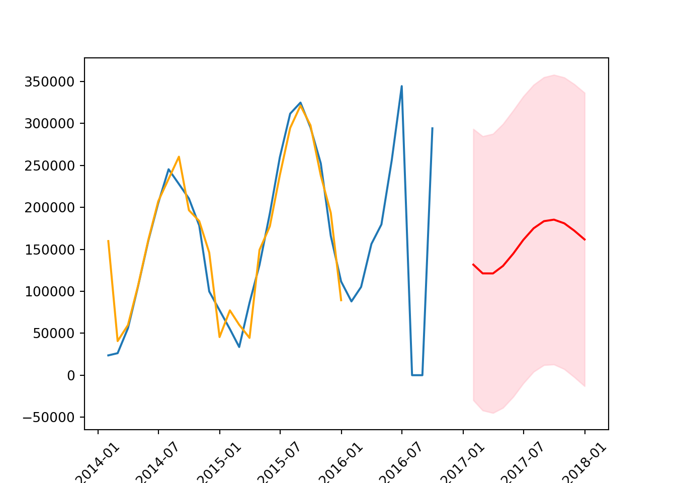
The forecast is more accurate than it was with AR(1) but needs to be shifted up a little to more accurately reflect the data. Additionally, the orange line is pretty accurately estimating the values.
# RMSE
mean_squared_error(test, forecast_mean, squared = False) # smaller or larger RMSE?
104316.4891780201
C:\Users\GEORGI~1\AppData\Local\Programs\Python\PYTHON~1\Lib\site-packages\sklearn\metrics\_regression.py:483: FutureWarning: 'squared' is deprecated in version 1.4 and will be removed in 1.6. To calculate the root mean squared error, use the function'root_mean_squared_error'.
warnings.warn(8.17 MA (Moving Average) model
The Moving Average (MA) model removes random movements from a time series model. Unlike models that rely solely on the historical values of the dataset (like the Autoregressive models), the MA model focuses on modeling the error term (residuals) of the predictions.
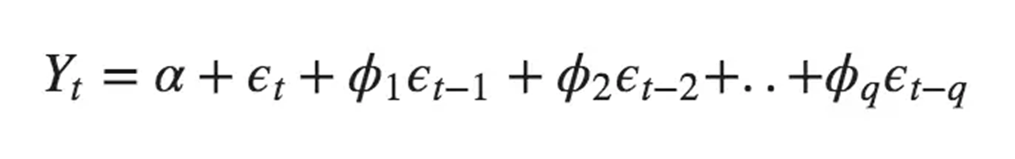
Where \(\alpha\) is the constants,
\(\phi\) is the parameters that need to be estimated (weight),
\(\epsilon\) is the white noise (error term)
8.17.1 MA(1)
# create the model
model = ARIMA(train, order = (0,0,1))
results = model.fit()
C:\Users\GEORGI~1\AppData\Local\Programs\Python\PYTHON~1\Lib\site-packages\statsmodels\tsa\statespace\sarimax.py:978: UserWarning: Non-invertible starting MA parameters found. Using zeros as starting parameters.
warn('Non-invertible starting MA parameters found.'results.summary()| Dep. Variable: | count | No. Observations: | 24 |
| Model: | ARIMA(0, 0, 1) | Log Likelihood | -298.997 |
| Date: | Mon, 22 Apr 2024 | AIC | 603.994 |
| Time: | 17:09:32 | BIC | 607.528 |
| Sample: | 01-31-2014 | HQIC | 604.931 |
| - 12-31-2015 | |||
| Covariance Type: | opg |
| coef | std err | z | P>|z| | [0.025 | 0.975] | |
| const | 1.598e+05 | 4.69e+04 | 3.405 | 0.001 | 6.78e+04 | 2.52e+05 |
| ma.L1 | 0.9058 | 0.793 | 1.142 | 0.253 | -0.649 | 2.460 |
| sigma2 | 6.595e+09 | 0.047 | 1.4e+11 | 0.000 | 6.6e+09 | 6.6e+09 |
| Ljung-Box (L1) (Q): | 14.58 | Jarque-Bera (JB): | 0.84 |
| Prob(Q): | 0.00 | Prob(JB): | 0.66 |
| Heteroskedasticity (H): | 1.31 | Skew: | 0.02 |
| Prob(H) (two-sided): | 0.71 | Kurtosis: | 2.08 |
Warnings:
[1] Covariance matrix calculated using the outer product of gradients (complex-step).
[2] Covariance matrix is singular or near-singular, with condition number 5.13e+27. Standard errors may be unstable.
Ljung-Box test - prob(Q) value of 0.00 suggests that there is no autocorrelation at lag 1, indicating good model fit.
Jarque-Bera test - prob(JB) value of 0.52 suggests that the residuals are normally distributed.
Heteroskedasticity test - prob(H) (two-sided) value of 0.60 suggests no significant heteroskedasticity, meaning the error variance is fairly constant.
# get forecast, means, confidence intervals
forecast = results.get_prediction(start = '2017-01-31', end = '2017-12-31')
forecast_mean = forecast.predicted_mean
confidence_intervals = forecast.conf_int()
# plot the data
plt.plot(series)
plt.plot(results.fittedvalues,
color = 'orange',
label = 'forecast')
plt.plot(forecast_mean, color = 'red')
plt.fill_between(forecast_mean.index,
confidence_intervals['lower count'],
confidence_intervals['upper count'],
color = 'pink',
alpha = 0.5)
plt.xticks(rotation = 45);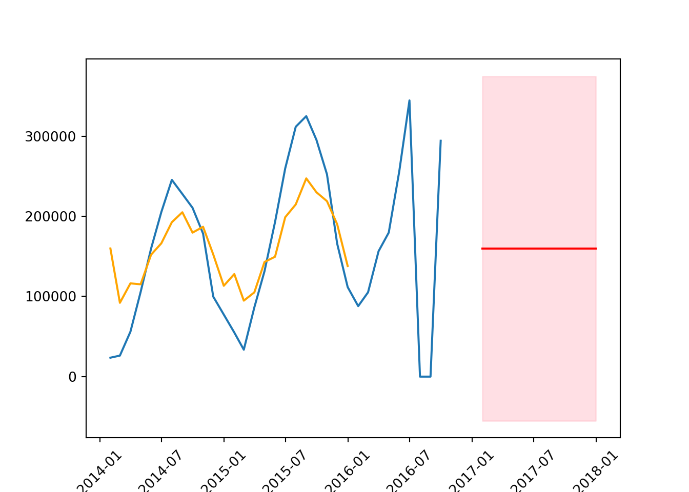
mean_squared_error(test, forecast_mean, squared = False)104874.51864512012
C:\Users\GEORGI~1\AppData\Local\Programs\Python\PYTHON~1\Lib\site-packages\sklearn\metrics\_regression.py:483: FutureWarning: 'squared' is deprecated in version 1.4 and will be removed in 1.6. To calculate the root mean squared error, use the function'root_mean_squared_error'.
warnings.warn(8.18 ARMA
This is a combination of the AR and MA models.
# create the model
model = ARIMA(train, order = (1,0,1))
results = model.fit()
results.summary()| Dep. Variable: | count | No. Observations: | 24 |
| Model: | ARIMA(1, 0, 1) | Log Likelihood | -285.879 |
| Date: | Mon, 22 Apr 2024 | AIC | 579.758 |
| Time: | 17:09:34 | BIC | 584.471 |
| Sample: | 01-31-2014 | HQIC | 581.009 |
| - 12-31-2015 | |||
| Covariance Type: | opg |
| coef | std err | z | P>|z| | [0.025 | 0.975] | |
| const | 1.598e+05 | 8.76e+04 | 1.825 | 0.068 | -1.18e+04 | 3.31e+05 |
| ar.L1 | 0.7809 | 0.357 | 2.190 | 0.029 | 0.082 | 1.480 |
| ma.L1 | 0.8630 | 0.413 | 2.089 | 0.037 | 0.053 | 1.673 |
| sigma2 | 1.969e+09 | 0.203 | 9.72e+09 | 0.000 | 1.97e+09 | 1.97e+09 |
| Ljung-Box (L1) (Q): | 2.57 | Jarque-Bera (JB): | 0.83 |
| Prob(Q): | 0.11 | Prob(JB): | 0.66 |
| Heteroskedasticity (H): | 1.67 | Skew: | -0.16 |
| Prob(H) (two-sided): | 0.48 | Kurtosis: | 2.15 |
Warnings:
[1] Covariance matrix calculated using the outer product of gradients (complex-step).
[2] Covariance matrix is singular or near-singular, with condition number 1.11e+27. Standard errors may be unstable.
# get forecast, means, confidence intervals
forecast = results.get_prediction(start = '2017-01-31', end = '2017-12-31')
forecast_mean = forecast.predicted_mean
confidence_intervals = forecast.conf_int()
# plot the data
plt.plot(series)
plt.plot(results.fittedvalues,
color = 'orange',
label = 'forecast')
plt.plot(forecast_mean, color = 'red')
plt.fill_between(forecast_mean.index,
confidence_intervals['lower count'],
confidence_intervals['upper count'],
color = 'pink',
alpha = 0.5)
plt.xticks(rotation = 45);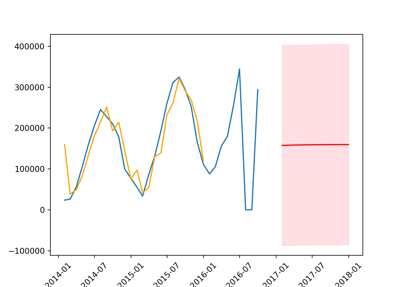
mean_squared_error(test, forecast_mean, squared = False)104947.85308784364
C:\Users\GEORGI~1\AppData\Local\Programs\Python\PYTHON~1\Lib\site-packages\sklearn\metrics\_regression.py:483: FutureWarning: 'squared' is deprecated in version 1.4 and will be removed in 1.6. To calculate the root mean squared error, use the function'root_mean_squared_error'.
warnings.warn(8.19 SARIMAX Model
The Seasonal AutoRegressive Integrated Moving Average with eXogenous variables model, or SARIMAX, is an extension of the ARIMA model used for time series forecasting. It incorporates both non-seasonal and seasonal elements, as well as external factors, making it particularly useful when the data show patterns not just at different times of the year but also when external variables influence the series.
The ‘X’ in SARIMAX stands for ‘exogenous variables’. These are external variables or predictors not part of the time series itself but can influence the target variable’s values. Including exogenous variables allows the model to account for factors that could impact the forecasting accuracy.
from statsmodels.tsa.statespace.sarimax import SARIMAXThe general model for SARIMAX is as follows:
SARIMAX(p, d, q)(P, D, Q)s
Non-Seasonal Components:
p: AutoRegressive order. Number of lag observations.
d: Degree of differencing. Number of times the data are differenced to achieve stationarity.
q: Moving Average order. Number of lagged forecast errors.
Seasonal Components:
P: Seasonal AutoRegressive order.
D: Seasonal differencing degree.
Q: Seasonal Moving Average order.
s: number of lags. For example, s=7 => we will use the values from one week ago to forecast the tomorrow’s value.
model = SARIMAX(endog=train,
              order=(1, 1, 1),
              seasonal_order=(1, 0, 0, 12)) # monthly data with annual cycle
results = model.fit()
C:\Users\GEORGI~1\AppData\Local\Programs\Python\PYTHON~1\Lib\site-packages\statsmodels\tsa\statespace\sarimax.py:997: UserWarning: Non-stationary starting seasonal autoregressive Using zeros as starting parameters.
warn('Non-stationary starting seasonal autoregressive'results.summary()| Dep. Variable: | count | No. Observations: | 24 |
| Model: | SARIMAX(1, 1, 1)x(1, 0, [], 12) | Log Likelihood | -267.575 |
| Date: | Mon, 22 Apr 2024 | AIC | 543.150 |
| Time: | 17:09:37 | BIC | 547.692 |
| Sample: | 01-31-2014 | HQIC | 544.293 |
| - 12-31-2015 | |||
| Covariance Type: | opg |
| coef | std err | z | P>|z| | [0.025 | 0.975] | |
| ar.L1 | 0.7066 | 0.445 | 1.587 | 0.113 | -0.166 | 1.579 |
| ma.L1 | 0.0768 | 0.789 | 0.097 | 0.922 | -1.470 | 1.623 |
| ar.S.L12 | 0.5016 | 0.379 | 1.324 | 0.185 | -0.241 | 1.244 |
| sigma2 | 9.846e+08 | 4.66e-10 | 2.11e+18 | 0.000 | 9.85e+08 | 9.85e+08 |
| Ljung-Box (L1) (Q): | 0.01 | Jarque-Bera (JB): | 0.01 |
| Prob(Q): | 0.91 | Prob(JB): | 1.00 |
| Heteroskedasticity (H): | 0.91 | Skew: | -0.01 |
| Prob(H) (two-sided): | 0.90 | Kurtosis: | 2.93 |
Warnings:
[1] Covariance matrix calculated using the outer product of gradients (complex-step).
[2] Covariance matrix is singular or near-singular, with condition number 3.17e+34. Standard errors may be unstable.
forecast = results.get_prediction(start = '2017-01-31', end = '2017-12-31')
forecast_mean = forecast.predicted_mean
confidence_intervals = forecast.conf_int()
plt.plot(series)
plt.plot(results.fittedvalues,
color = 'orange',
label = 'forecast')
plt.plot(forecast_mean, color = 'red')
plt.fill_between(forecast_mean.index,
confidence_intervals['lower count'],
confidence_intervals['upper count'],
color = 'pink',
alpha = 0.5)
plt.xticks(rotation = 45);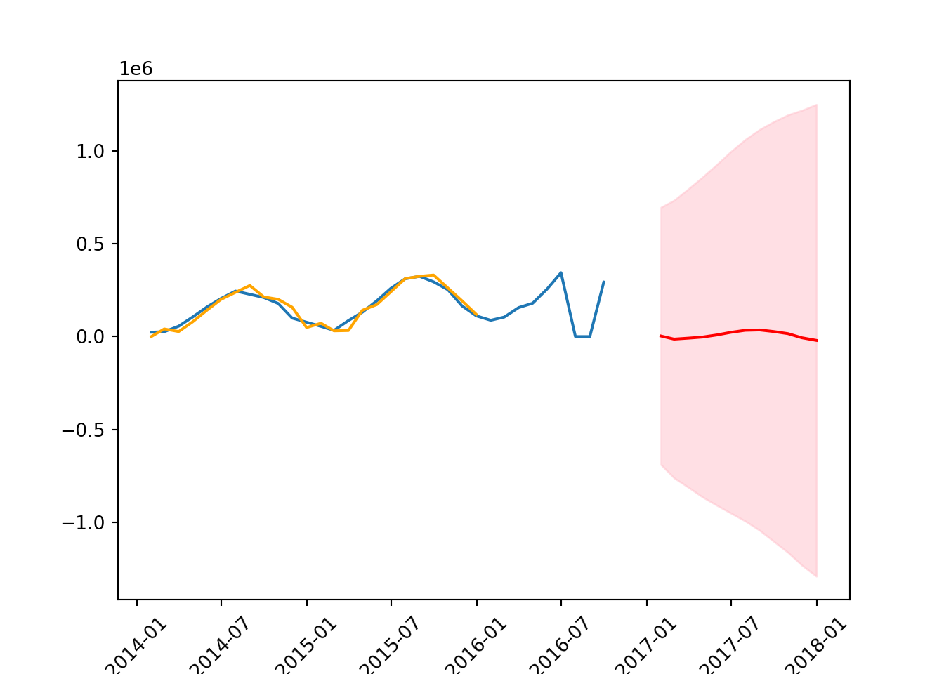
mean_squared_error(test, forecast_mean, squared = False)185672.92610518975
C:\Users\GEORGI~1\AppData\Local\Programs\Python\PYTHON~1\Lib\site-packages\sklearn\metrics\_regression.py:483: FutureWarning: 'squared' is deprecated in version 1.4 and will be removed in 1.6. To calculate the root mean squared error, use the function'root_mean_squared_error'.
warnings.warn(8.20 Auto ARIMA
Auto ARIMA manually selects the best ARIMA model by evaluating various combinations of parameters.
It automates the following steps: 1. It tests the stationarity of the data and applies the necessary differencing to make the series stationary. 2. It iteratively explores different combinations of p, d, and q values (and also P, D, Q for seasonal data) to find the best model according to a given criterion, usually the AIC (Akaike Information Criterion), BIC (Bayesian Information Criterion), or similar. 3. Once the best parameters are identified, it fits the ARIMA model to the data, allowing for predictions to be made.
import pmdarima as pmdDocumentation: https://alkaline-ml.com/pmdarima/modules/generated/pmdarima.arima.auto_arima.html
We need to set up an initial range for the series, with the following parameters:
# set up parameters
results = pmd.auto_arima(series,
                         start_p=0,  # initial guess for AR(p)
                         start_d=0,  # initial guess for I(d)
                         start_q=0,  # initial guess for MA(q)
                         max_p=5,    # max guess for AR(p)
                         max_d=2,    # max guess for I(d)
                         max_q=5,    # max guess for MA(q)
                         m=12,        # seasonal order
                         start_P=0,  # initial guess for seasonal AR(P)
                         start_D=0,  # initial guess for seasonal I(D)
                         start_Q=0,  # initial guess for seasonal MA(Q)
                         max_P = 3,
                         max_D = 1,
                         max_Q = 3,
                         information_criterion='bic',
                         trace=True,
                         error_action='ignore',
                         stepwise = False
                         )
ARIMA(0,0,0)(0,1,0)[12] intercept : BIC=553.755, Time=0.01 sec
ARIMA(0,0,0)(0,1,1)[12] intercept : BIC=555.356, Time=0.27 sec
ARIMA(0,0,0)(0,1,2)[12] intercept : BIC=556.037, Time=0.09 sec
ARIMA(0,0,0)(0,1,3)[12] intercept : BIC=558.952, Time=0.15 sec
ARIMA(0,0,0)(1,1,0)[12] intercept : BIC=556.615, Time=0.02 sec
ARIMA(0,0,0)(1,1,1)[12] intercept : BIC=557.199, Time=0.05 sec
ARIMA(0,0,0)(1,1,2)[12] intercept : BIC=558.958, Time=0.12 sec
ARIMA(0,0,0)(1,1,3)[12] intercept : BIC=561.996, Time=0.42 sec
ARIMA(0,0,0)(2,1,0)[12] intercept : BIC=555.865, Time=0.04 sec
ARIMA(0,0,0)(2,1,1)[12] intercept : BIC=558.900, Time=0.10 sec
ARIMA(0,0,0)(2,1,2)[12] intercept : BIC=561.925, Time=0.74 sec
ARIMA(0,0,0)(2,1,3)[12] intercept : BIC=564.903, Time=1.33 sec
ARIMA(0,0,0)(3,1,0)[12] intercept : BIC=558.907, Time=0.14 sec
ARIMA(0,0,0)(3,1,1)[12] intercept : BIC=561.795, Time=0.48 sec
ARIMA(0,0,0)(3,1,2)[12] intercept : BIC=564.840, Time=0.32 sec
ARIMA(0,0,1)(0,1,0)[12] intercept : BIC=545.422, Time=0.02 sec
ARIMA(0,0,1)(0,1,1)[12] intercept : BIC=547.185, Time=0.04 sec
ARIMA(0,0,1)(0,1,2)[12] intercept : BIC=549.993, Time=0.51 sec
ARIMA(0,0,1)(0,1,3)[12] intercept : BIC=552.946, Time=0.91 sec
ARIMA(0,0,1)(1,1,0)[12] intercept : BIC=547.866, Time=0.03 sec
ARIMA(0,0,1)(1,1,1)[12] intercept : BIC=550.087, Time=0.10 sec
ARIMA(0,0,1)(1,1,2)[12] intercept : BIC=552.998, Time=0.85 sec
ARIMA(0,0,1)(1,1,3)[12] intercept : BIC=555.989, Time=0.41 sec
ARIMA(0,0,1)(2,1,0)[12] intercept : BIC=549.900, Time=0.08 sec
ARIMA(0,0,1)(2,1,1)[12] intercept : BIC=552.944, Time=0.12 sec
ARIMA(0,0,1)(2,1,2)[12] intercept : BIC=555.986, Time=0.20 sec
ARIMA(0,0,1)(3,1,0)[12] intercept : BIC=552.945, Time=0.60 sec
ARIMA(0,0,1)(3,1,1)[12] intercept : BIC=inf, Time=2.36 sec
ARIMA(0,0,2)(0,1,0)[12] intercept : BIC=549.947, Time=0.02 sec
ARIMA(0,0,2)(0,1,1)[12] intercept : BIC=552.429, Time=0.04 sec
ARIMA(0,0,2)(0,1,2)[12] intercept : BIC=555.136, Time=0.27 sec
ARIMA(0,0,2)(0,1,3)[12] intercept : BIC=558.092, Time=0.17 sec
ARIMA(0,0,2)(1,1,0)[12] intercept : BIC=552.821, Time=0.05 sec
ARIMA(0,0,2)(1,1,1)[12] intercept : BIC=555.301, Time=0.07 sec
ARIMA(0,0,2)(1,1,2)[12] intercept : BIC=558.123, Time=0.16 sec
ARIMA(0,0,2)(2,1,0)[12] intercept : BIC=555.038, Time=0.32 sec
ARIMA(0,0,2)(2,1,1)[12] intercept : BIC=558.083, Time=0.20 sec
ARIMA(0,0,2)(3,1,0)[12] intercept : BIC=558.083, Time=0.18 sec
ARIMA(0,0,3)(0,1,0)[12] intercept : BIC=554.455, Time=0.03 sec
ARIMA(0,0,3)(0,1,1)[12] intercept : BIC=555.979, Time=0.07 sec
ARIMA(0,0,3)(0,1,2)[12] intercept : BIC=559.018, Time=0.53 sec
ARIMA(0,0,3)(1,1,0)[12] intercept : BIC=556.558, Time=0.06 sec
ARIMA(0,0,3)(1,1,1)[12] intercept : BIC=559.023, Time=0.10 sec
ARIMA(0,0,3)(2,1,0)[12] intercept : BIC=559.067, Time=0.30 sec
ARIMA(0,0,4)(0,1,0)[12] intercept : BIC=571.587, Time=0.13 sec
ARIMA(0,0,4)(0,1,1)[12] intercept : BIC=574.537, Time=0.11 sec
ARIMA(0,0,4)(1,1,0)[12] intercept : BIC=574.620, Time=0.09 sec
ARIMA(0,0,5)(0,1,0)[12] intercept : BIC=inf, Time=0.48 sec
ARIMA(1,0,0)(0,1,0)[12] intercept : BIC=551.230, Time=0.01 sec
ARIMA(1,0,0)(0,1,1)[12] intercept : BIC=553.951, Time=0.03 sec
ARIMA(1,0,0)(0,1,2)[12] intercept : BIC=556.015, Time=0.07 sec
ARIMA(1,0,0)(0,1,3)[12] intercept : BIC=559.030, Time=0.16 sec
ARIMA(1,0,0)(1,1,0)[12] intercept : BIC=554.246, Time=0.03 sec
ARIMA(1,0,0)(1,1,1)[12] intercept : BIC=556.421, Time=0.25 sec
ARIMA(1,0,0)(1,1,2)[12] intercept : BIC=559.012, Time=0.11 sec
ARIMA(1,0,0)(1,1,3)[12] intercept : BIC=562.025, Time=0.31 sec
ARIMA(1,0,0)(2,1,0)[12] intercept : BIC=555.983, Time=0.28 sec
ARIMA(1,0,0)(2,1,1)[12] intercept : BIC=559.022, Time=0.19 sec
ARIMA(1,0,0)(2,1,2)[12] intercept : BIC=562.053, Time=0.19 sec
ARIMA(1,0,0)(3,1,0)[12] intercept : BIC=559.027, Time=1.40 sec
ARIMA(1,0,0)(3,1,1)[12] intercept : BIC=561.988, Time=0.54 sec
ARIMA(1,0,1)(0,1,0)[12] intercept : BIC=548.423, Time=0.03 sec
ARIMA(1,0,1)(0,1,1)[12] intercept : BIC=550.163, Time=0.10 sec
ARIMA(1,0,1)(0,1,2)[12] intercept : BIC=552.935, Time=0.18 sec
ARIMA(1,0,1)(0,1,3)[12] intercept : BIC=555.859, Time=0.49 sec
ARIMA(1,0,1)(1,1,0)[12] intercept : BIC=550.877, Time=0.08 sec
ARIMA(1,0,1)(1,1,1)[12] intercept : BIC=553.050, Time=0.25 sec
ARIMA(1,0,1)(1,1,2)[12] intercept : BIC=555.929, Time=0.36 sec
ARIMA(1,0,1)(2,1,0)[12] intercept : BIC=552.812, Time=0.18 sec
ARIMA(1,0,1)(2,1,1)[12] intercept : BIC=555.856, Time=0.40 sec
ARIMA(1,0,1)(3,1,0)[12] intercept : BIC=555.856, Time=0.57 sec
ARIMA(1,0,2)(0,1,0)[12] intercept : BIC=552.576, Time=0.05 sec
ARIMA(1,0,2)(0,1,1)[12] intercept : BIC=555.270, Time=0.12 sec
ARIMA(1,0,2)(0,1,2)[12] intercept : BIC=557.765, Time=0.58 sec
ARIMA(1,0,2)(1,1,0)[12] intercept : BIC=555.517, Time=0.09 sec
ARIMA(1,0,2)(1,1,1)[12] intercept : BIC=558.065, Time=0.55 sec
ARIMA(1,0,2)(2,1,0)[12] intercept : BIC=557.590, Time=1.03 sec
ARIMA(1,0,3)(0,1,0)[12] intercept : BIC=555.851, Time=0.07 sec
ARIMA(1,0,3)(0,1,1)[12] intercept : BIC=557.725, Time=0.11 sec
ARIMA(1,0,3)(1,1,0)[12] intercept : BIC=558.368, Time=0.12 sec
ARIMA(1,0,4)(0,1,0)[12] intercept : BIC=572.657, Time=0.09 sec
ARIMA(2,0,0)(0,1,0)[12] intercept : BIC=548.138, Time=0.21 sec
ARIMA(2,0,0)(0,1,1)[12] intercept : BIC=549.821, Time=0.06 sec
ARIMA(2,0,0)(0,1,2)[12] intercept : BIC=551.091, Time=0.10 sec
ARIMA(2,0,0)(0,1,3)[12] intercept : BIC=553.832, Time=0.19 sec
ARIMA(2,0,0)(1,1,0)[12] intercept : BIC=550.850, Time=0.06 sec
ARIMA(2,0,0)(1,1,1)[12] intercept : BIC=551.857, Time=0.14 sec
ARIMA(2,0,0)(1,1,2)[12] intercept : BIC=553.810, Time=0.35 sec
ARIMA(2,0,0)(2,1,0)[12] intercept : BIC=550.770, Time=0.13 sec
ARIMA(2,0,0)(2,1,1)[12] intercept : BIC=553.777, Time=0.36 sec
ARIMA(2,0,0)(3,1,0)[12] intercept : BIC=553.791, Time=0.23 sec
ARIMA(2,0,1)(0,1,0)[12] intercept : BIC=551.133, Time=0.03 sec
ARIMA(2,0,1)(0,1,1)[12] intercept : BIC=552.500, Time=0.08 sec
ARIMA(2,0,1)(0,1,2)[12] intercept : BIC=555.179, Time=0.16 sec
ARIMA(2,0,1)(1,1,0)[12] intercept : BIC=553.550, Time=0.27 sec
ARIMA(2,0,1)(1,1,1)[12] intercept : BIC=555.330, Time=1.57 sec
ARIMA(2,0,1)(2,1,0)[12] intercept : BIC=554.934, Time=0.18 sec
ARIMA(2,0,2)(0,1,0)[12] intercept : BIC=553.736, Time=0.18 sec
ARIMA(2,0,2)(0,1,1)[12] intercept : BIC=556.490, Time=0.40 sec
ARIMA(2,0,2)(1,1,0)[12] intercept : BIC=557.533, Time=0.36 sec
ARIMA(2,0,3)(0,1,0)[12] intercept : BIC=inf, Time=0.39 sec
ARIMA(3,0,0)(0,1,0)[12] intercept : BIC=551.084, Time=0.03 sec
ARIMA(3,0,0)(0,1,1)[12] intercept : BIC=552.271, Time=0.07 sec
ARIMA(3,0,0)(0,1,2)[12] intercept : BIC=554.879, Time=0.11 sec
ARIMA(3,0,0)(1,1,0)[12] intercept : BIC=553.497, Time=0.07 sec
ARIMA(3,0,0)(1,1,1)[12] intercept : BIC=555.057, Time=0.14 sec
ARIMA(3,0,0)(2,1,0)[12] intercept : BIC=554.623, Time=0.27 sec
ARIMA(3,0,1)(0,1,0)[12] intercept : BIC=553.896, Time=0.04 sec
ARIMA(3,0,1)(0,1,1)[12] intercept : BIC=555.532, Time=0.10 sec
ARIMA(3,0,1)(1,1,0)[12] intercept : BIC=556.593, Time=0.12 sec
ARIMA(3,0,2)(0,1,0)[12] intercept : BIC=558.666, Time=0.65 sec
ARIMA(4,0,0)(0,1,0)[12] intercept : BIC=552.920, Time=0.54 sec
ARIMA(4,0,0)(0,1,1)[12] intercept : BIC=555.075, Time=0.09 sec
ARIMA(4,0,0)(1,1,0)[12] intercept : BIC=555.957, Time=0.14 sec
ARIMA(4,0,1)(0,1,0)[12] intercept : BIC=555.939, Time=0.17 sec
ARIMA(5,0,0)(0,1,0)[12] intercept : BIC=inf, Time=0.37 sec
Best model: ARIMA(0,0,1)(0,1,0)[12] intercept
Total fit time: 31.329 secondsresults.summary()| Dep. Variable: | y | No. Observations: | 33 |
| Model: | SARIMAX(0, 0, 1)x(0, 1, [], 12) | Log Likelihood | -268.144 |
| Date: | Mon, 22 Apr 2024 | AIC | 542.288 |
| Time: | 17:10:16 | BIC | 545.422 |
| Sample: | 01-31-2014 | HQIC | 542.969 |
| - 09-30-2016 | |||
| Covariance Type: | opg |
| coef | std err | z | P>|z| | [0.025 | 0.975] | |
| intercept | -4801.0683 | 7.38e+04 | -0.065 | 0.948 | -1.49e+05 | 1.4e+05 |
| ma.L1 | 0.8545 | 0.665 | 1.286 | 0.199 | -0.448 | 2.157 |
| sigma2 | 8.615e+09 | 1.679 | 5.13e+09 | 0.000 | 8.62e+09 | 8.62e+09 |
| Ljung-Box (L1) (Q): | 0.02 | Jarque-Bera (JB): | 224.79 |
| Prob(Q): | 0.88 | Prob(JB): | 0.00 |
| Heteroskedasticity (H): | 28.91 | Skew: | -3.87 |
| Prob(H) (two-sided): | 0.00 | Kurtosis: | 17.03 |
Warnings:
[1] Covariance matrix calculated using the outer product of gradients (complex-step).
[2] Covariance matrix is singular or near-singular, with condition number 1.23e+25. Standard errors may be unstable.
We can then use what was suggested to us by AutoARIMA.
model = SARIMAX(endog=train,
              order=(1, 0, 0),
              seasonal_order=(0, 1, 0, 12), # same as what has been suggested to us
                trend = 'c' #the intercept
               )
results = model.fit()
# get the forecast, mean, and confidence intervals
forecast = results.get_prediction(start = '2017-01-31', end = '2017-12-31')
forecast_mean = forecast.predicted_mean
confidence_intervals = forecast.conf_int()plt.plot(series)
plt.plot(results.fittedvalues,
color = 'orange',
label = 'forecast')
plt.plot(forecast_mean, color = 'red')
plt.fill_between(forecast_mean.index,
confidence_intervals['lower count'],
confidence_intervals['upper count'],
color = 'pink',
alpha = 0.5)
plt.xticks(rotation = 45);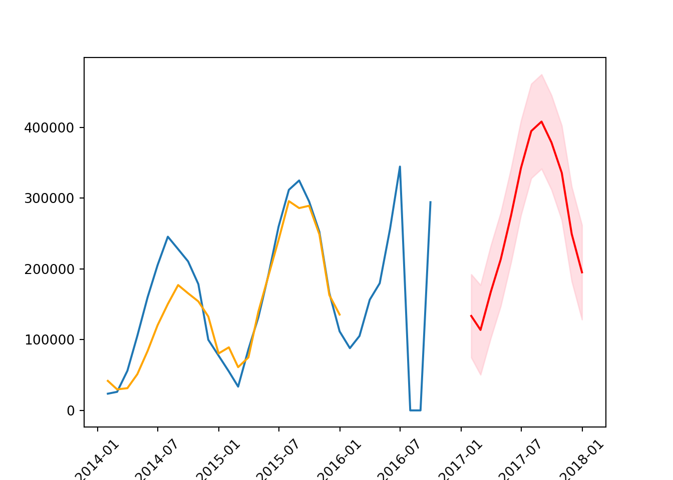
mean_squared_error(test, forecast_mean, squared = False)171857.73541525897
C:\Users\GEORGI~1\AppData\Local\Programs\Python\PYTHON~1\Lib\site-packages\sklearn\metrics\_regression.py:483: FutureWarning: 'squared' is deprecated in version 1.4 and will be removed in 1.6. To calculate the root mean squared error, use the function'root_mean_squared_error'.
warnings.warn(8.21 Prophet
Prophet is a forecasting tool designed by Facebook’s Core Data Science team. It’s built for making forecasts for univariate time series datasets that have strong seasonal patterns and historical data. Prophet is especially useful in cases where data is affected by seasonality and other holidays or events.
The model works well with daily observations that display patterns on different time scales. It also handles missing data and trend changes well, making it robust for a variety of use cases. One of the key features of Prophet is its ability to handle the effects of holidays and special events by including them as additional regressors, thus improving the accuracy of forecasts.
8.21.1 Key Features:
- Easy to Use: Prophet requires minimal tuning and can be used straight out of the box for many forecasting tasks.
- Robust to Missing Data: It can handle missing data and outliers with little to no preprocessing.
- Flexibility: The model parameters can be easily adjusted to tune the forecast for specific needs.
- Handles Seasonality: Prophet automatically detects and forecasts seasonalities at different levels (daily, weekly, yearly).
- Holiday Effects: It can include holidays and special events, improving forecast accuracy around these times.
Prophet is based on an additive model where non-linear trends are fit with yearly, weekly, and daily seasonality, plus holiday effects.
It uses three main model components: trend, seasonality, and holidays. The trend models non-periodic changes, seasonality represents periodic changes, and holidays incorporate the effects of holidays and events.
8.21.2 Introduction to the data
# view of data
bicycles.head()
starttime stoptime tripduration temperature
0 2014-06-30 23:57:00 2014-07-01 00:07:00 10.066667 68.0
1 2014-06-30 23:56:00 2014-07-01 00:00:00 4.383333 68.0
2 2014-06-30 23:33:00 2014-06-30 23:35:00 2.100000 68.0
3 2014-06-30 23:26:00 2014-07-01 00:24:00 58.016667 68.0
4 2014-06-30 23:16:00 2014-06-30 23:26:00 10.633333 68.0# information about the data
bicycles.info()<class 'pandas.core.frame.DataFrame'>
RangeIndex: 9495235 entries, 0 to 9495234
Data columns (total 4 columns):
# Column Dtype
--- ------ -----
0 starttime object
1 stoptime object
2 tripduration float64
3 temperature float64
dtypes: float64(2), object(2)
memory usage: 289.8+ MB8.21.3 Data preprocessing
# convert starttime to datetime column
bicycles['starttime'] = pd.to_datetime(bicycles['starttime'], format ='%Y-%m-%d %H:%M:%S')bicycles.info()<class 'pandas.core.frame.DataFrame'>
RangeIndex: 9495235 entries, 0 to 9495234
Data columns (total 4 columns):
# Column Dtype
--- ------ -----
0 starttime datetime64[ns]
1 stoptime object
2 tripduration float64
3 temperature float64
dtypes: datetime64[ns](1), float64(2), object(1)
memory usage: 289.8+ MB# create a new column which picks out date from starttime
bicycles['starttime_date'] = bicycles['starttime'].dt.date
bicycles.head() starttime stoptime ... temperature starttime_date
0 2014-06-30 23:57:00 2014-07-01 00:07:00 ... 68.0 2014-06-30
1 2014-06-30 23:56:00 2014-07-01 00:00:00 ... 68.0 2014-06-30
2 2014-06-30 23:33:00 2014-06-30 23:35:00 ... 68.0 2014-06-30
3 2014-06-30 23:26:00 2014-07-01 00:24:00 ... 68.0 2014-06-30
4 2014-06-30 23:16:00 2014-06-30 23:26:00 ... 68.0 2014-06-30
[5 rows x 5 columns]8.21.4 Resampling
# create a dataframe
df = pd.DataFrame()
# group by starttime_date column
grouped_data = bicycles.groupby('starttime_date')
# create column to count occurrences
df['count'] = grouped_data['starttime'].count()
# create column to sum the trip durations
df['trip_duration_sum'] = grouped_data['tripduration'].sum()
# create column for mean of temperature
df['temperature_avg'] = grouped_data['temperature'].mean()
df.head() count trip_duration_sum temperature_avg
starttime_date
2014-01-01 95 1020.183333 19.483158
2014-01-02 111 1292.850000 16.833333
2014-01-03 6 58.383333 -5.633333
2014-01-04 181 2001.350000 30.007735
2014-01-05 32 393.133333 16.756250# plot the count column
df['count'].plot()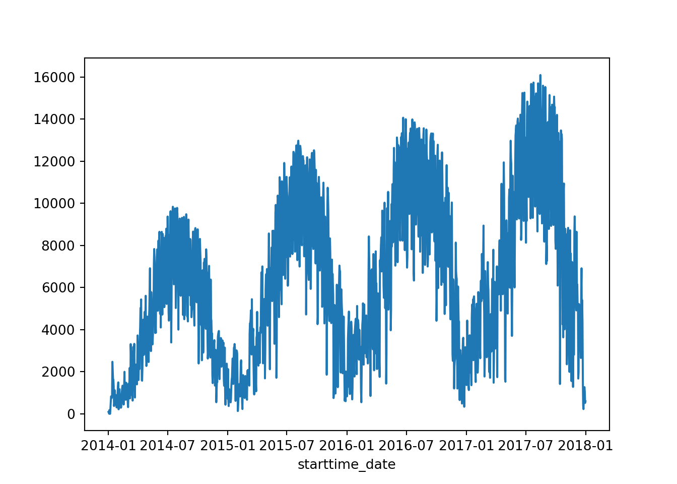
# reset the index
df.reset_index(inplace = True)
df.head()
starttime_date count trip_duration_sum temperature_avg
0 2014-01-01 95 1020.183333 19.483158
1 2014-01-02 111 1292.850000 16.833333
2 2014-01-03 6 58.383333 -5.633333
3 2014-01-04 181 2001.350000 30.007735
4 2014-01-05 32 393.133333 16.756250# set starttime_date column to datetime
df['starttime_date'] = pd.to_datetime(df['starttime_date'], format ='%Y-%m-%d')# create a new df with number of trips
number_trips = df[['starttime_date','count']]
number_trips.head() starttime_date count
0 2014-01-01 95
1 2014-01-02 111
2 2014-01-03 6
3 2014-01-04 181
4 2014-01-05 328.21.5 Train-test split
# define training data
train = number_trips.iloc[:-365]
train.tail()
starttime_date count
1088 2016-12-27 2521
1089 2016-12-28 3167
1090 2016-12-29 2858
1091 2016-12-30 2651
1092 2016-12-31 1669train.shape(1093, 2)# define test data
test = number_trips.iloc[-365:]
test.shape(365, 2)8.21.6 Baseline Model
# name the columns for train and test dataframes
train.columns = ['ds', 'y']
test.columns = ['ds', 'y']
These are named like so because:
“The input to Prophet is always a dataframe with two columns: ds and y. The ds (datestamp) column should be of a format expected by Pandas, ideally YYYY-MM-DD for a date or YYYY-MM-DD HH:MM:SS for a timestamp. The y column must be numeric, and represents the measurement we wish to forecast.”
train.head() ds y
0 2014-01-01 95
1 2014-01-02 111
2 2014-01-03 6
3 2014-01-04 181
4 2014-01-05 32Create the model
from prophet import Prophet
import plotly
Using the method fit(), Prophet analyses the data and isolates both the seasonality and trend.
model = Prophet()

model.fit(train)
<prophet.forecaster.Prophet object at 0x000001B55D9473E0>
17:11:07 - cmdstanpy - INFO - Chain [1] start processing
17:11:07 - cmdstanpy - INFO - Chain [1] done processingForecast
The make_future_dataframe() method creates a DataFrame with the future dates. It requires us to specify the number of future values to predict, and the frequency of the data.
# make dataframe with future dates
future = model.make_future_dataframe(periods = 365, freq = 'D') # 365 days
future
ds
0 2014-01-01
1 2014-01-02
2 2014-01-03
3 2014-01-04
4 2014-01-05
... ...
1453 2017-12-27
1454 2017-12-28
1455 2017-12-29
1456 2017-12-30
1457 2017-12-31
[1458 rows x 1 columns]By default it will also include the dates from the history.
The predict method will assign each row in future a predicted value which it names yhat. In statistics, y hat (\(\hat{y}\)) is the term given to the estimated or predicted values in a regression or other predictive model.
If you pass in historical dates, it will provide an in-sample fit (data that is used to fit or train a model).
# predict future values
forecast = model.predict(future)

forecast.tail() # use tail to view the future dates
ds trend ... multiplicative_terms_upper yhat
1453 2017-12-27 6953.411794 ... 0.0 3357.108019
1454 2017-12-28 6952.371031 ... 0.0 3223.978213
1455 2017-12-29 6951.330267 ... 0.0 2888.235697
1456 2017-12-30 6950.289504 ... 0.0 705.616709
1457 2017-12-31 6949.248741 ... 0.0 399.459810
[5 rows x 19 columns]The predicted values are in the last column, yhat - in this case it will be the predicted number of trips each day.
yearly shows the model’s estimation of the annual trend in the data.
yearly_lower and yearly_upper provide the lower and upper bounds of the yearly component’s uncertainty interval. They indicate the range within which the actual yearly trend is expected to lie, with a certain level of confidence. If these values are very close to yearly, then the range will be small.
# plot the model
fig = model.plot(forecast, xlabel = 'Days', ylabel = 'Number of rented bicycles')
C:\Users\GEORGI~1\AppData\Local\Programs\Python\PYTHON~1\Lib\site-packages\prophet\plot.py:72: FutureWarning: The behavior of DatetimeProperties.to_pydatetime is deprecated, in a future version this will return a Series containing python datetime objects instead of an ndarray. To retain the old behavior, call `np.array` on the result
fcst_t = fcst['ds'].dt.to_pydatetime()
C:\Users\GEORGI~1\AppData\Local\Programs\Python\PYTHON~1\Lib\site-packages\prophet\plot.py:73: FutureWarning: The behavior of DatetimeProperties.to_pydatetime is deprecated, in a future version this will return a Series containing python datetime objects instead of an ndarray. To retain the old behavior, call `np.array` on the result
ax.plot(m.history['ds'].dt.to_pydatetime(), m.history['y'], 'k.',plt.title('Daily bicycle renting')
plt.plot(test['ds'], test['y'], color = 'red', alpha = 0.25)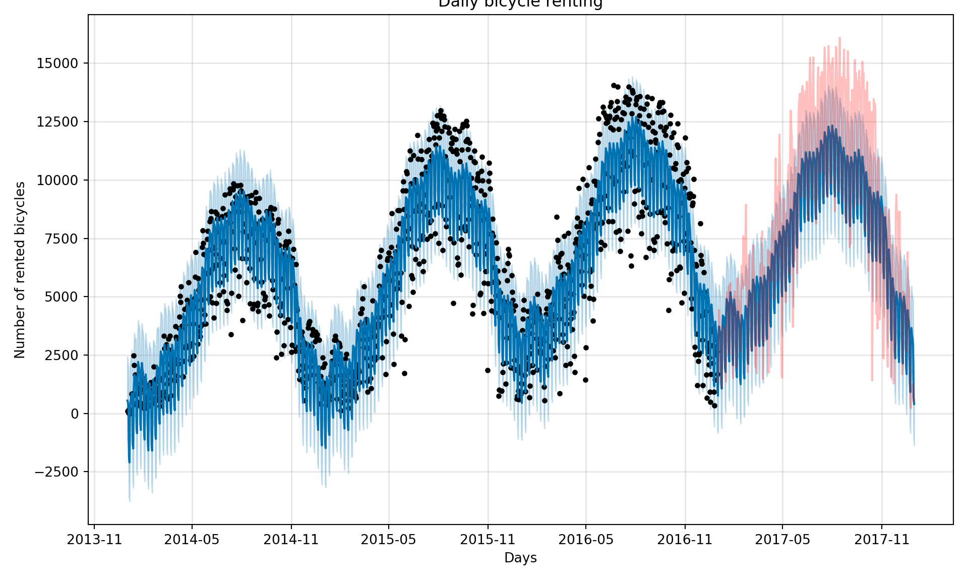
- the black dots represent the actual data points (original data)
- the dark blue lines are the estimated values from the model
- the light blue lines are the margins of errors
- the red represents the region of the forecasting predictions - the red is the actual values and the blue is the prediction.
Evaluate
First we need to select the y_hat column from the forecasting dataframe.
y_predicted = forecast['yhat'].iloc[-365:] # select just the last values, using negative indexing

y_predicted
1093 757.162419
1094 3158.704571
1095 3724.404468
1096 3535.537909
1097 3523.732882
...
1453 3357.108019
1454 3223.978213
1455 2888.235697
1456 705.616709
1457 399.459810
Name: yhat, Length: 365, dtype: float64# calculating the RMSE
mean_squared_error(test['y'], y_predicted, squared = False)2233.9296019296426
C:\Users\GEORGI~1\AppData\Local\Programs\Python\PYTHON~1\Lib\site-packages\sklearn\metrics\_regression.py:483: FutureWarning: 'squared' is deprecated in version 1.4 and will be removed in 1.6. To calculate the root mean squared error, use the function'root_mean_squared_error'.
warnings.warn(Lastly, we can create some visualisations based on the information from the model. It will show us the forecasted trend, the weekly trend and yearly trend.
# plot visualisations
fig = model.plot_components(forecast)
C:\Users\GEORGI~1\AppData\Local\Programs\Python\PYTHON~1\Lib\site-packages\prophet\plot.py:228: FutureWarning: The behavior of DatetimeProperties.to_pydatetime is deprecated, in a future version this will return a Series containing python datetime objects instead of an ndarray. To retain the old behavior, call `np.array` on the result
fcst_t = fcst['ds'].dt.to_pydatetime()
C:\Users\GEORGI~1\AppData\Local\Programs\Python\PYTHON~1\Lib\site-packages\prophet\plot.py:351: FutureWarning: The behavior of DatetimeProperties.to_pydatetime is deprecated, in a future version this will return a Series containing python datetime objects instead of an ndarray. To retain the old behavior, call `np.array` on the result
df_y['ds'].dt.to_pydatetime(), seas[name], ls='-', c='#0072B2')
C:\Users\GEORGI~1\AppData\Local\Programs\Python\PYTHON~1\Lib\site-packages\prophet\plot.py:354: FutureWarning: The behavior of DatetimeProperties.to_pydatetime is deprecated, in a future version this will return a Series containing python datetime objects instead of an ndarray. To retain the old behavior, call `np.array` on the result
df_y['ds'].dt.to_pydatetime(), seas[name + '_lower'],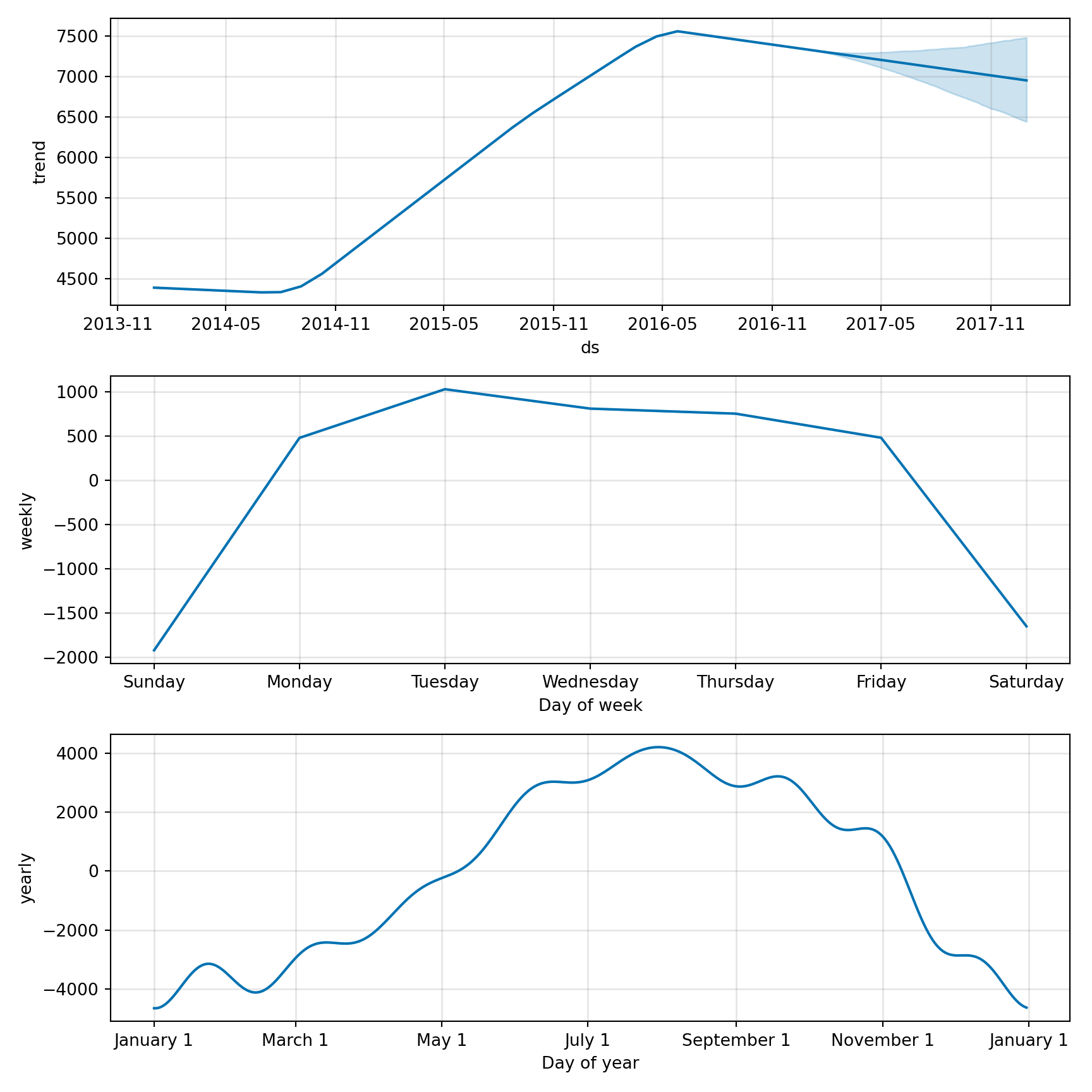
8.21.7 The components of the Prophet model
# plot of the data
train['y'].plot()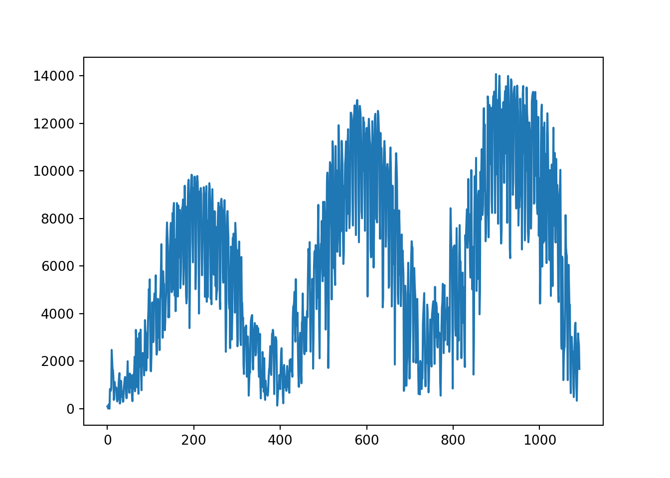
The trend can be:
linear(
linear) - straight lines with positive or negative slope between the changepoints.constant(
flat) - a constant trendlogistic(
logistic) - the trend is a logistic non linear function.
The seasonality and other predictors can be additive or multiplicative.
The additive model: y(t) = g(t) + s(t) + h(t) + r(t) + Et
The multiplicative model: y(t) = g(t) x (1 + s(t)) + h(t) + r(t) + Et)
- y(t) - the prediction
- g(t) - the trend
- s(t) - the seasonality
- h(t) - the holidays
- r(t) - other predictors
- Et - the white noise term
The main parameters of the Prophet model are the following:
yearly_seasonality: True or False if there is or there isn’t yearly seasonality. It can also be a number which represents the Fourier order with which the component is aproximated(default 10).
weekly_seasonality: True or False if there is or there isn’t weekly seasonality. It can also be a number which represents the Fourier order with which the component is aproximated(default 3).
daily_seasonality(if the data is hourly or more granular): True or False if there is or there isn’t daily seasonality. It can also be a number which represents the Fourier order with which the component is aproximated(default 4).
n_changepoints: number of trend changepoints.
changepoints: list of explicit changepoint dates, where trend changes are made.
changepoint_range: percentage of the data where changepoints are inferred.
changepoint_prior_scale: the strength or possibility of trend change. The bigger the value, the higher the flexibility of the trend.
seasonality_prior_scale: strength of the seasonality component or components. This value can be general for all the seasonalities or adjusted specifically for each of them.
holiday_prior_scale: strength of the holiday component.
8.21.8 Fourier Order
A Fourier series is a sum of sine waves.
The Fourier order in the Prophet model determines the complexity of seasonal patterns it can fit. A lower Fourier order means the model will capture broader, more general seasonal trends. A higher Fourier order allows the model to fit more intricate and frequent variations within a season. The choice of Fourier order is crucial as it balances the model’s flexibility against the risk of overfitting to the noise in the data.
We could add some parameters to the Prophet model - in this case seasonality_mode and yearly_seasonality.
model = Prophet(seasonality_mode = 'multiplicative',
                yearly_seasonality = 15)
model.fit(train)
<prophet.forecaster.Prophet object at 0x000001B555E9BA10>
17:11:14 - cmdstanpy - INFO - Chain [1] start processing
17:11:14 - cmdstanpy - INFO - Chain [1] done processingfuture = model.make_future_dataframe(periods = 306, freq = 'D')
forecast = model.predict(future)fig = model.plot(forecast, xlabel = 'Days', ylabel = 'Number of rented bicycles')C:\Users\GEORGI~1\AppData\Local\Programs\Python\PYTHON~1\Lib\site-packages\prophet\plot.py:72: FutureWarning: The behavior of DatetimeProperties.to_pydatetime is deprecated, in a future version this will return a Series containing python datetime objects instead of an ndarray. To retain the old behavior, call `np.array` on the result
fcst_t = fcst['ds'].dt.to_pydatetime()
C:\Users\GEORGI~1\AppData\Local\Programs\Python\PYTHON~1\Lib\site-packages\prophet\plot.py:73: FutureWarning: The behavior of DatetimeProperties.to_pydatetime is deprecated, in a future version this will return a Series containing python datetime objects instead of an ndarray. To retain the old behavior, call `np.array` on the result
ax.plot(m.history['ds'].dt.to_pydatetime(), m.history['y'], 'k.',plt.title('Daily bicycle renting')
plt.plot(test['ds'], test['y'], color = 'red', alpha = 0.5)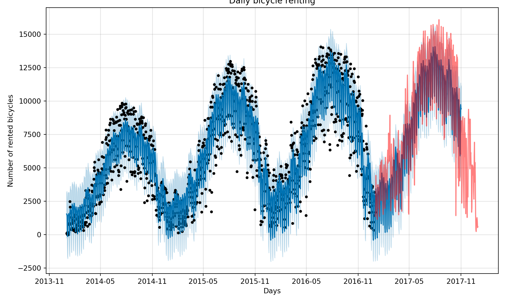
The estimated values are fitted better to the actual values than they were in the previous model.
y_predicted = forecast['yhat'].iloc[-365:]
mean_squared_error(test['y'], y_predicted, squared = False)
4895.080496875805
C:\Users\GEORGI~1\AppData\Local\Programs\Python\PYTHON~1\Lib\site-packages\sklearn\metrics\_regression.py:483: FutureWarning: 'squared' is deprecated in version 1.4 and will be removed in 1.6. To calculate the root mean squared error, use the function'root_mean_squared_error'.
warnings.warn(fig = model.plot_components(forecast)C:\Users\GEORGI~1\AppData\Local\Programs\Python\PYTHON~1\Lib\site-packages\prophet\plot.py:228: FutureWarning: The behavior of DatetimeProperties.to_pydatetime is deprecated, in a future version this will return a Series containing python datetime objects instead of an ndarray. To retain the old behavior, call `np.array` on the result
fcst_t = fcst['ds'].dt.to_pydatetime()
C:\Users\GEORGI~1\AppData\Local\Programs\Python\PYTHON~1\Lib\site-packages\prophet\plot.py:351: FutureWarning: The behavior of DatetimeProperties.to_pydatetime is deprecated, in a future version this will return a Series containing python datetime objects instead of an ndarray. To retain the old behavior, call `np.array` on the result
df_y['ds'].dt.to_pydatetime(), seas[name], ls='-', c='#0072B2')
C:\Users\GEORGI~1\AppData\Local\Programs\Python\PYTHON~1\Lib\site-packages\prophet\plot.py:354: FutureWarning: The behavior of DatetimeProperties.to_pydatetime is deprecated, in a future version this will return a Series containing python datetime objects instead of an ndarray. To retain the old behavior, call `np.array` on the result
df_y['ds'].dt.to_pydatetime(), seas[name + '_lower'],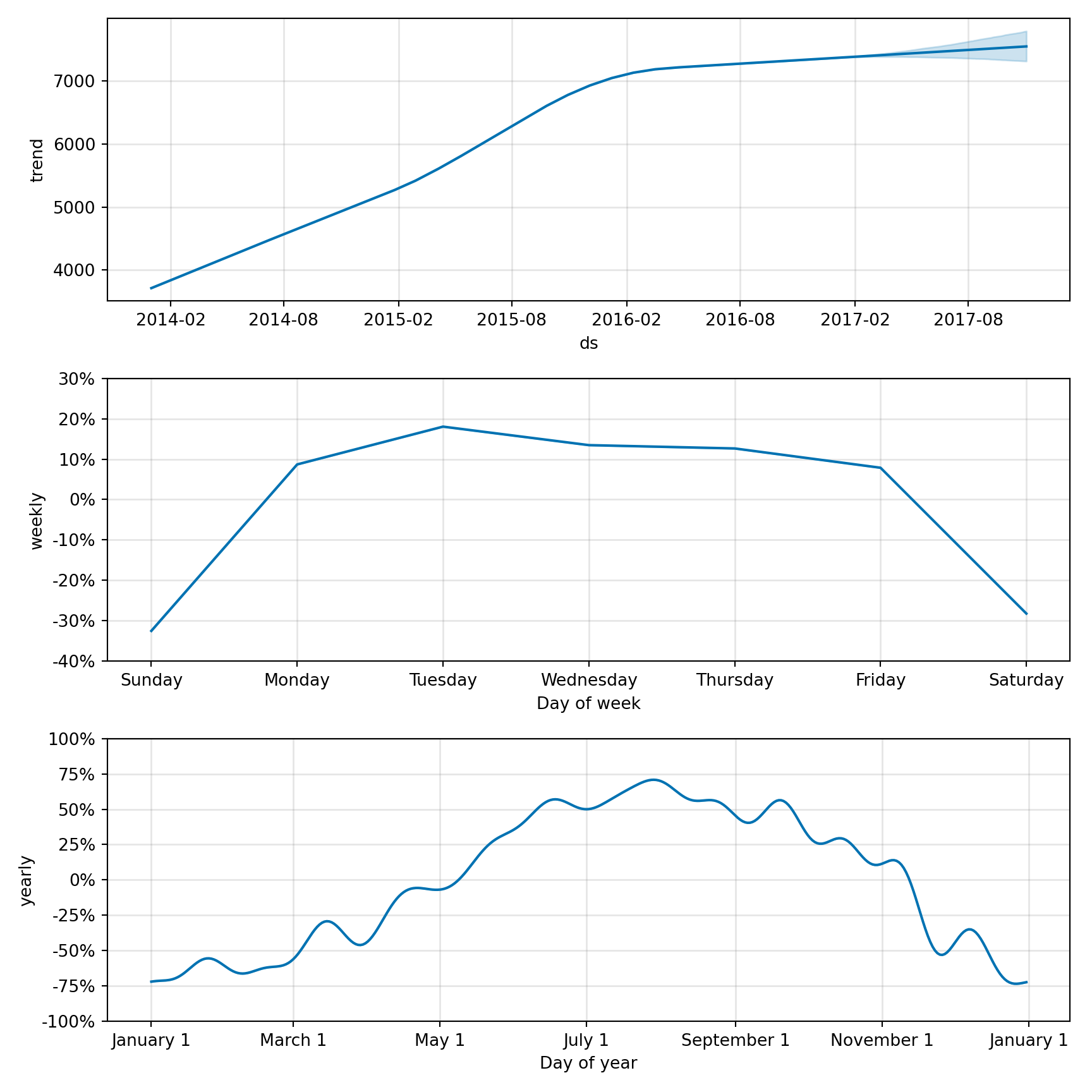
8.21.9 Seasonal Analysis
You may need to investigate a little further to help you understand the seasonalities. - annual seasonality - monthly seasonality - weekly seasonality - other seasonalities
# extract the days from the 'starttime_date' column
df['day'] = df['starttime_date'].dt.dayofweek
We can create the below plot to separate the days of the week.
# plot visualisation
fig, ax = plt.subplots(figsize=(15,6))
day_order = range(6)
sns.scatterplot(x="starttime_date",
                y="count",
                hue="day",
                hue_order=day_order,
                data=df,
                ax=ax)

# 0-Monday --- 6-Sunday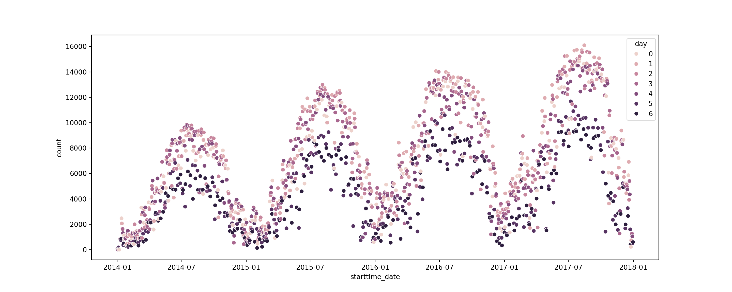
We have more trips during the working days than at the weekend. Also, the data shows that in the summer there is a considerable distance in the number of trips between the working days and the weekends. However, in the winter of 2015, the number of trips from the working days and weekends a close to each other, and 2016 and 2017 show a higher variation in the number of trips on the winter days.
# group by day
df.groupby(df['day'])['count'].sum()
day
0 1476647
1 1590726
2 1538038
3 1530674
4 1458457
5 979440
6 921253
Name: count, dtype: int64# extract year
df['year'] = df['starttime_date'].dt.year
# extract month
df['month'] = df['starttime_date'].dt.month
# group by the year and the month
df_ym = df.groupby(['year', 'month'])['count'].sum().reset_index()
df_ym.head() year month count
0 2014 1 23617
1 2014 2 26221
2 2014 3 56020
3 2014 4 105428
4 2014 5 159957# plot the dataframe
fig, ax = plt.subplots(figsize=(15, 6))
ax = sns.lineplot(x = df_ym['month'], y = df_ym['count'], hue=df_ym['year'], ax=ax)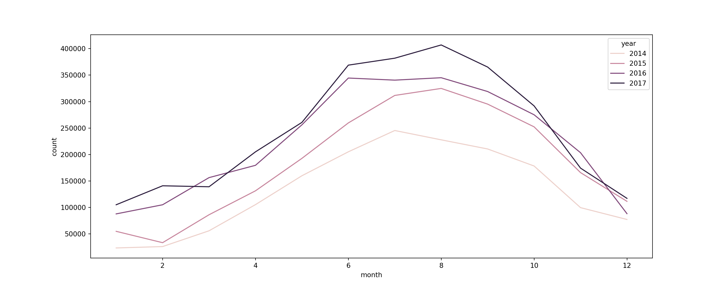
In the plot above we see a decrease in the winter months and increase in the summer months. Also can be noticed a growing trend from year to year.
The weekly seasonality changes after the winter of 2015 (we can use the conditional seasonality)
To do: - Load the holidays - Define the conditional seasonality - Use other predictors
8.21.10 Conditional Seasonality
Conditional seasonality refers to seasonal patterns in your data that only happen under certain conditions.
Example: Imagine a coffee shop that sells more hot chocolate in the winter than in the summer. That’s a seasonal pattern. If this coffee shop is inside a ski resort, they might sell even more hot chocolate, but only when it’s the skiing season. That’s conditional seasonality – where the seasonality of hot chocolate sales is conditional on whether it’s the ski season or not.
Prophet asks for two complementary boolean columns, one that is True if the condition is met and False elsewhere, and a second column that is the opposite. We will consider the 1st of March 2015 a change in the seasonality.
# define conditional seasonality
df['weekly_before_march_2015'] = [True if dt < pd.to_datetime('2015-03-01') else False for dt in df['starttime_date']]
df['weekly_after_march_2015'] = [False if dt < pd.to_datetime('2015-03-01') else True for dt in df['starttime_date']]
We will implement this below.
8.21.11 Other regressors
df.columnsIndex(['starttime_date', 'count', 'trip_duration_sum', 'temperature_avg',
'day', 'year', 'month', 'weekly_before_march_2015',
'weekly_after_march_2015'],
dtype='object')# mean and standard deviation of temperature
print(df['temperature_avg'].mean())53.101448172284215print(df['temperature_avg'].std())21.00291171776019# view the correlation of count and temperature average - is the number of bicyles rented correlated with the temperature?
df[['count','temperature_avg']].corr() count temperature_avg
count 1.000000 0.777235
temperature_avg 0.777235 1.0000008.21.12 Building the model
Preprocessing
df.columnsIndex(['starttime_date', 'count', 'trip_duration_sum', 'temperature_avg',
'day', 'year', 'month', 'weekly_before_march_2015',
'weekly_after_march_2015'],
dtype='object')We need to rename starttime_date to ds and count to y. The naming convention of ds and y is a design choice made by the creators of Prophet to standardize the input format. This way, the model knows exactly where to look for the data it needs to function, without the user having to specify the names of the input columns each time they fit a model.
# rename the columns
renamed_columns = ['ds', 'y', 'trip_duration_sum', 'temperature_avg',
       'day', 'year', 'month', 'weekly_before_march_2015',
       'weekly_after_march_2015']
df.columns = renamed_columns
df.head() ds y ... weekly_before_march_2015 weekly_after_march_2015
0 2014-01-01 95 ... True False
1 2014-01-02 111 ... True False
2 2014-01-03 6 ... True False
3 2014-01-04 181 ... True False
4 2014-01-05 32 ... True False
[5 rows x 9 columns]# define train
train = df.iloc[:-365] # all data except the last 365 rows
train.shape(1093, 9)# define test
test = df.iloc[-365:] # the last 365 rows onwards
test.shape(365, 9)The model
# define the model
model = Prophet(seasonality_mode = 'multiplicative',
               growth = 'linear',
               yearly_seasonality = False,
                weekly_seasonality = False,
                daily_seasonality = False
               )

# 'additive' - by default
Add the holidays
To add the holidays to the model we need to: 1. create the model 2. add model.add_country_holidays(country_name = ‘US’) 3. Fit the model 4. All the usual steps
import holidays
# view holidays for a specific country
uk_holidays = holidays.UnitedKingdom()
uk_holidaysholidays.country_holidays('GB')# For UK holidays in the year 2022 - there were lots of holidays in this year
uk_holidays_2022 = holidays.UnitedKingdom(years=[2022])
uk_holidays_2022{datetime.date(2022, 4, 15): 'Good Friday', datetime.date(2022, 5, 2): 'May Day', datetime.date(2022, 6, 2): 'Spring Bank Holiday', datetime.date(2022, 6, 3): 'Platinum Jubilee of Elizabeth II', datetime.date(2022, 9, 19): 'State Funeral of Queen Elizabeth II', datetime.date(2022, 1, 1): "New Year's Day", datetime.date(2022, 1, 3): "New Year's Day (observed)", datetime.date(2022, 12, 25): 'Christmas Day', datetime.date(2022, 12, 27): 'Christmas Day (observed)', datetime.date(2022, 12, 26): 'Boxing Day'}# add the holidays to the model
model.add_country_holidays(country_name = 'GB')<prophet.forecaster.Prophet object at 0x000001B5622350A0>This page contains a link to all of the codes for each country. -
8.21.12.1 Seasonalities
# add yearly seasonality to the model
model.add_seasonality(name = 'yearly',
period = 365,
fourier_order = 20)<prophet.forecaster.Prophet object at 0x000001B5622350A0># add monthly seasonality to the model
model.add_seasonality(name = 'monthly',
period = 31,
fourier_order = 7)<prophet.forecaster.Prophet object at 0x000001B5622350A0>8.21.12.2 Choose Fourier order values:
- Yearly Seasonality: For yearly seasonality, starting with a Fourier order of 10-20 can be a good rule of thumb for annual data. Adjust based on the complexity of the seasonal pattern.
- Weekly/Daily Seasonality: For weekly or daily seasonality, the required Fourier order might be lower. Start with values like 3-7 for weekly seasonality or higher for daily if your data has multiple peaks within a week.
train.columnsIndex(['ds', 'y', 'trip_duration_sum', 'temperature_avg', 'day', 'year',
'month', 'weekly_before_march_2015', 'weekly_after_march_2015'],
dtype='object')# add conditional seasonality
model.add_seasonality(name = 'weekly_before_march_2015',
period = 7,
fourier_order = 2, # smaller gaps - less important
condition_name = 'weekly_before_march_2015')<prophet.forecaster.Prophet object at 0x000001B5622350A0># add conditional seasonality
model.add_seasonality(name = 'weekly_after_march_2015',
period = 7,
fourier_order = 4,
condition_name = 'weekly_after_march_2015')<prophet.forecaster.Prophet object at 0x000001B5622350A0># add the temperature
model.add_regressor('temperature_avg')<prophet.forecaster.Prophet object at 0x000001B5622350A0>Fit the model
model.fit(train[['ds', 'y', 'weekly_before_march_2015','weekly_after_march_2015', 'temperature_avg']]) # just the important columns<prophet.forecaster.Prophet object at 0x000001B5622350A0>
17:11:41 - cmdstanpy - INFO - Chain [1] start processing
17:11:41 - cmdstanpy - INFO - Chain [1] done processingNow we follow the same steps.
Predict
future = model.make_future_dataframe(periods = 365, freq = 'D')
future ds
0 2014-01-01
1 2014-01-02
2 2014-01-03
3 2014-01-04
4 2014-01-05
... ...
1453 2017-12-27
1454 2017-12-28
1455 2017-12-29
1456 2017-12-30
1457 2017-12-31
[1458 rows x 1 columns]# create some new columns for the dataframe
# input values from existing dataframe
future[['weekly_before_march_2015',
'weekly_after_march_2015',
'temperature_avg']] = df[['weekly_before_march_2015',
'weekly_after_march_2015',
'temperature_avg']]
future ds ... temperature_avg
0 2014-01-01 ... 19.483158
1 2014-01-02 ... 16.833333
2 2014-01-03 ... -5.633333
3 2014-01-04 ... 30.007735
4 2014-01-05 ... 16.756250
... ... ... ...
1453 2017-12-27 ... 2.458013
1454 2017-12-28 ... 10.802762
1455 2017-12-29 ... 12.978932
1456 2017-12-30 ... 3.657033
1457 2017-12-31 ... 8.657167
[1458 rows x 4 columns]forecast = model.predict(future)
forecast.tail() ds trend ... additive_terms_upper yhat
1453 2017-12-27 7399.951421 ... 0.0 464.920898
1454 2017-12-28 7400.508065 ... 0.0 1361.049891
1455 2017-12-29 7401.064710 ... 0.0 1485.257011
1456 2017-12-30 7401.621354 ... 0.0 -2182.473371
1457 2017-12-31 7402.177998 ... 0.0 -2298.337998
[5 rows x 58 columns]fig = model.plot(forecast, xlabel = 'Days', ylabel = 'Number of rented bicycles')C:\Users\GEORGI~1\AppData\Local\Programs\Python\PYTHON~1\Lib\site-packages\prophet\plot.py:72: FutureWarning: The behavior of DatetimeProperties.to_pydatetime is deprecated, in a future version this will return a Series containing python datetime objects instead of an ndarray. To retain the old behavior, call `np.array` on the result
fcst_t = fcst['ds'].dt.to_pydatetime()
C:\Users\GEORGI~1\AppData\Local\Programs\Python\PYTHON~1\Lib\site-packages\prophet\plot.py:73: FutureWarning: The behavior of DatetimeProperties.to_pydatetime is deprecated, in a future version this will return a Series containing python datetime objects instead of an ndarray. To retain the old behavior, call `np.array` on the result
ax.plot(m.history['ds'].dt.to_pydatetime(), m.history['y'], 'k.',plt.title('Daily bicycle renting')
plt.plot(test['ds'], test['y'], color = 'red', alpha = 0.5)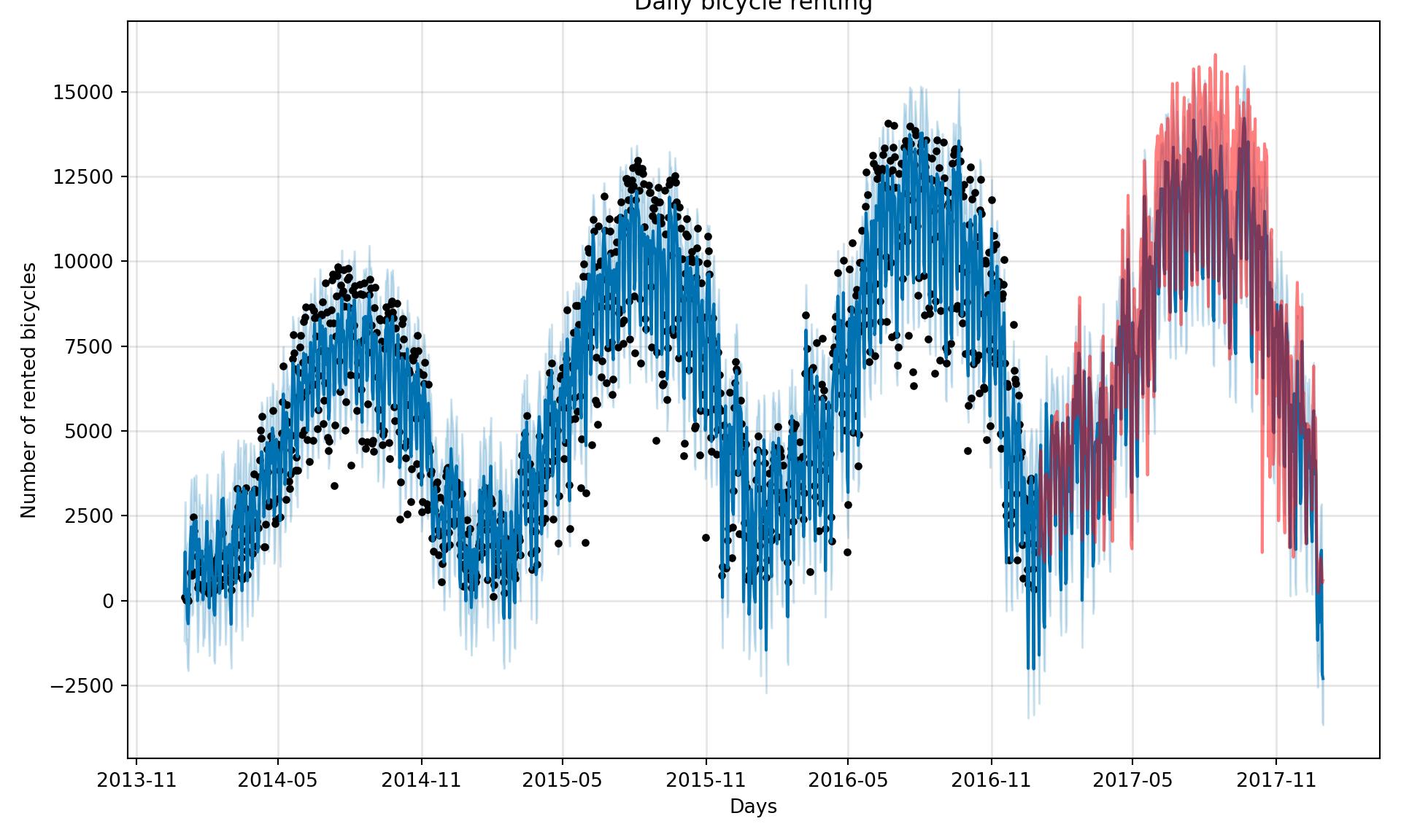
Again this has slightly improved.
y_predicted = forecast['yhat'].iloc[-365:]
mean_squared_error(test['y'], y_predicted, squared = False)1690.776235057746
C:\Users\GEORGI~1\AppData\Local\Programs\Python\PYTHON~1\Lib\site-packages\sklearn\metrics\_regression.py:483: FutureWarning: 'squared' is deprecated in version 1.4 and will be removed in 1.6. To calculate the root mean squared error, use the function'root_mean_squared_error'.
warnings.warn(fig = model.plot_components(forecast)C:\Users\GEORGI~1\AppData\Local\Programs\Python\PYTHON~1\Lib\site-packages\prophet\plot.py:228: FutureWarning: The behavior of DatetimeProperties.to_pydatetime is deprecated, in a future version this will return a Series containing python datetime objects instead of an ndarray. To retain the old behavior, call `np.array` on the result
fcst_t = fcst['ds'].dt.to_pydatetime()
C:\Users\GEORGI~1\AppData\Local\Programs\Python\PYTHON~1\Lib\site-packages\prophet\plot.py:351: FutureWarning: The behavior of DatetimeProperties.to_pydatetime is deprecated, in a future version this will return a Series containing python datetime objects instead of an ndarray. To retain the old behavior, call `np.array` on the result
df_y['ds'].dt.to_pydatetime(), seas[name], ls='-', c='#0072B2')
C:\Users\GEORGI~1\AppData\Local\Programs\Python\PYTHON~1\Lib\site-packages\prophet\plot.py:354: FutureWarning: The behavior of DatetimeProperties.to_pydatetime is deprecated, in a future version this will return a Series containing python datetime objects instead of an ndarray. To retain the old behavior, call `np.array` on the result
df_y['ds'].dt.to_pydatetime(), seas[name + '_lower'],
C:\Users\GEORGI~1\AppData\Local\Programs\Python\PYTHON~1\Lib\site-packages\prophet\plot.py:397: FutureWarning: The behavior of DatetimeProperties.to_pydatetime is deprecated, in a future version this will return a Series containing python datetime objects instead of an ndarray. To retain the old behavior, call `np.array` on the result
artists += ax.plot(df_y['ds'].dt.to_pydatetime(), seas[name], ls='-',
C:\Users\GEORGI~1\AppData\Local\Programs\Python\PYTHON~1\Lib\site-packages\prophet\plot.py:401: FutureWarning: The behavior of DatetimeProperties.to_pydatetime is deprecated, in a future version this will return a Series containing python datetime objects instead of an ndarray. To retain the old behavior, call `np.array` on the result
df_y['ds'].dt.to_pydatetime(), seas[name + '_lower'],
C:\Users\GEORGI~1\AppData\Local\Programs\Python\PYTHON~1\Lib\site-packages\prophet\plot.py:228: FutureWarning: The behavior of DatetimeProperties.to_pydatetime is deprecated, in a future version this will return a Series containing python datetime objects instead of an ndarray. To retain the old behavior, call `np.array` on the result
fcst_t = fcst['ds'].dt.to_pydatetime()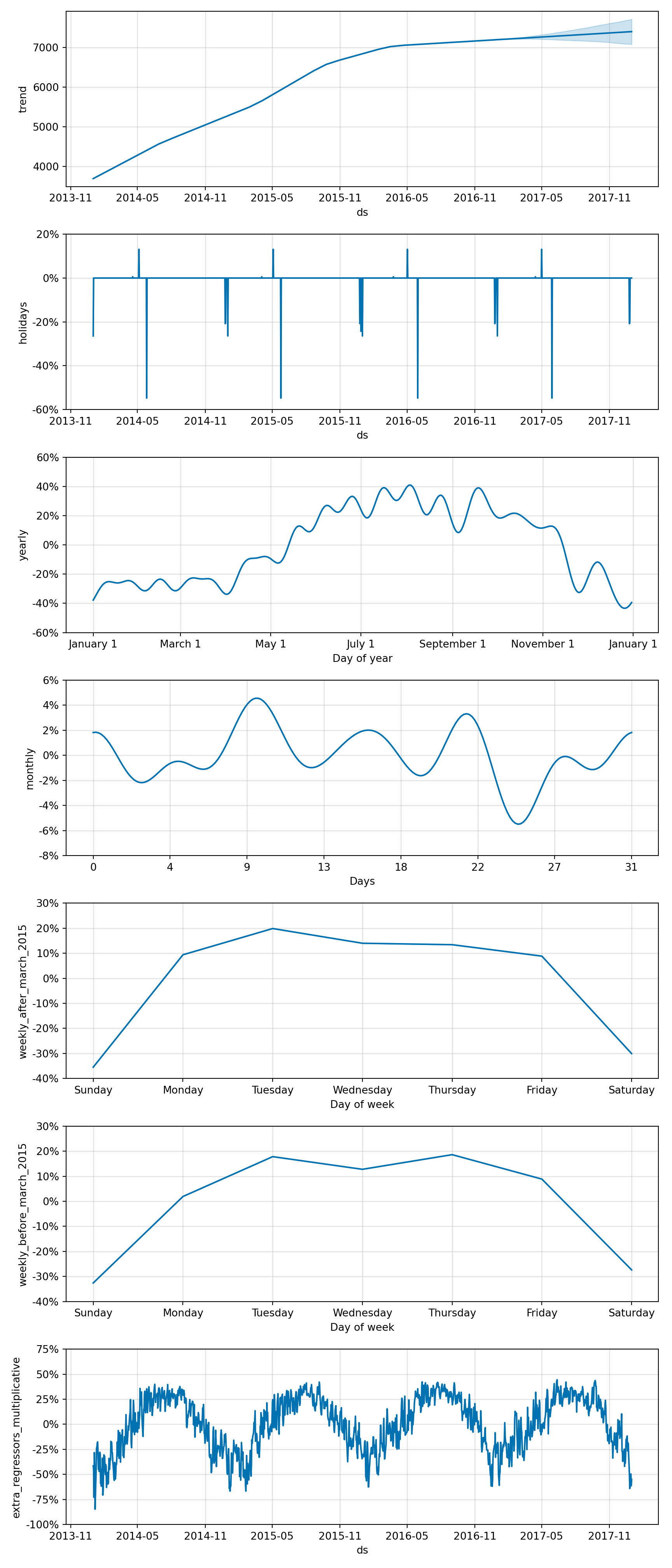
8.21.12.3 Hyperparameters
We may be able to get the model to perform better if we set up a specific combination of the parameters for the Fourier order.
Note: There are no code outputs in this section, purely just to try and save some memory! You will need to run the code on your own to view the output.
from sklearn.model_selection import ParameterGrid<sklearn.model_selection._search.ParameterGrid object at 0x000001B5C0C0E7E0>[{'weekly_seasonality': 3, 'yearly_seasonality': 10}, {'weekly_seasonality': 3, 'yearly_seasonality': 11}, {'weekly_seasonality': 3, 'yearly_seasonality': 12}, {'weekly_seasonality': 3, 'yearly_seasonality': 13}, {'weekly_seasonality': 3, 'yearly_seasonality': 14}, {'weekly_seasonality': 3, 'yearly_seasonality': 15}, {'weekly_seasonality': 3, 'yearly_seasonality': 16}, {'weekly_seasonality': 3, 'yearly_seasonality': 17}, {'weekly_seasonality': 3, 'yearly_seasonality': 18}, {'weekly_seasonality': 3, 'yearly_seasonality': 19}, {'weekly_seasonality': 4, 'yearly_seasonality': 10}, {'weekly_seasonality': 4, 'yearly_seasonality': 11}, {'weekly_seasonality': 4, 'yearly_seasonality': 12}, {'weekly_seasonality': 4, 'yearly_seasonality': 13}, {'weekly_seasonality': 4, 'yearly_seasonality': 14}, {'weekly_seasonality': 4, 'yearly_seasonality': 15}, {'weekly_seasonality': 4, 'yearly_seasonality': 16}, {'weekly_seasonality': 4, 'yearly_seasonality': 17}, {'weekly_seasonality': 4, 'yearly_seasonality': 18}, {'weekly_seasonality': 4, 'yearly_seasonality': 19}]We want to create a dataframe that contains all of the possible combinations for our parameters, and the corresponding RMSE value.
<prophet.forecaster.Prophet object at 0x000001B5C055EE40>
<prophet.forecaster.Prophet object at 0x000001B562337800>
<prophet.forecaster.Prophet object at 0x000001B5C056D280>
<prophet.forecaster.Prophet object at 0x000001B5C0BACD70>
<prophet.forecaster.Prophet object at 0x000001B5C0952360>
<prophet.forecaster.Prophet object at 0x000001B5C0950A70>
<prophet.forecaster.Prophet object at 0x000001B5C077E030>
<prophet.forecaster.Prophet object at 0x000001B562337800>
<prophet.forecaster.Prophet object at 0x000001B5C0B36990>
<prophet.forecaster.Prophet object at 0x000001B5C07EF230>
<prophet.forecaster.Prophet object at 0x000001B5C0B36B70>
<prophet.forecaster.Prophet object at 0x000001B56217E240>
<prophet.forecaster.Prophet object at 0x000001B5C077E030>
<prophet.forecaster.Prophet object at 0x000001B55130D670>
<prophet.forecaster.Prophet object at 0x000001B5C0790B00>
<prophet.forecaster.Prophet object at 0x000001B562213BF0>
<prophet.forecaster.Prophet object at 0x000001B5C0B76510>
<prophet.forecaster.Prophet object at 0x000001B5C0814800>
<prophet.forecaster.Prophet object at 0x000001B562241AF0>
<prophet.forecaster.Prophet object at 0x000001B556A0FC80>
17:11:48 - cmdstanpy - INFO - Chain [1] start processing
17:11:48 - cmdstanpy - INFO - Chain [1] done processing
C:\Users\GEORGI~1\AppData\Local\Programs\Python\PYTHON~1\Lib\site-packages\sklearn\metrics\_regression.py:483: FutureWarning: 'squared' is deprecated in version 1.4 and will be removed in 1.6. To calculate the root mean squared error, use the function'root_mean_squared_error'.
warnings.warn(
17:11:49 - cmdstanpy - INFO - Chain [1] start processing
17:11:49 - cmdstanpy - INFO - Chain [1] done processing
C:\Users\GEORGI~1\AppData\Local\Programs\Python\PYTHON~1\Lib\site-packages\sklearn\metrics\_regression.py:483: FutureWarning: 'squared' is deprecated in version 1.4 and will be removed in 1.6. To calculate the root mean squared error, use the function'root_mean_squared_error'.
warnings.warn(
17:11:50 - cmdstanpy - INFO - Chain [1] start processing
17:11:50 - cmdstanpy - INFO - Chain [1] done processing
C:\Users\GEORGI~1\AppData\Local\Programs\Python\PYTHON~1\Lib\site-packages\sklearn\metrics\_regression.py:483: FutureWarning: 'squared' is deprecated in version 1.4 and will be removed in 1.6. To calculate the root mean squared error, use the function'root_mean_squared_error'.
warnings.warn(
17:11:50 - cmdstanpy - INFO - Chain [1] start processing
17:11:51 - cmdstanpy - INFO - Chain [1] done processing
C:\Users\GEORGI~1\AppData\Local\Programs\Python\PYTHON~1\Lib\site-packages\sklearn\metrics\_regression.py:483: FutureWarning: 'squared' is deprecated in version 1.4 and will be removed in 1.6. To calculate the root mean squared error, use the function'root_mean_squared_error'.
warnings.warn(
17:11:51 - cmdstanpy - INFO - Chain [1] start processing
17:11:51 - cmdstanpy - INFO - Chain [1] done processing
C:\Users\GEORGI~1\AppData\Local\Programs\Python\PYTHON~1\Lib\site-packages\sklearn\metrics\_regression.py:483: FutureWarning: 'squared' is deprecated in version 1.4 and will be removed in 1.6. To calculate the root mean squared error, use the function'root_mean_squared_error'.
warnings.warn(
17:11:52 - cmdstanpy - INFO - Chain [1] start processing
17:11:52 - cmdstanpy - INFO - Chain [1] done processing
C:\Users\GEORGI~1\AppData\Local\Programs\Python\PYTHON~1\Lib\site-packages\sklearn\metrics\_regression.py:483: FutureWarning: 'squared' is deprecated in version 1.4 and will be removed in 1.6. To calculate the root mean squared error, use the function'root_mean_squared_error'.
warnings.warn(
17:11:53 - cmdstanpy - INFO - Chain [1] start processing
17:11:53 - cmdstanpy - INFO - Chain [1] done processing
C:\Users\GEORGI~1\AppData\Local\Programs\Python\PYTHON~1\Lib\site-packages\sklearn\metrics\_regression.py:483: FutureWarning: 'squared' is deprecated in version 1.4 and will be removed in 1.6. To calculate the root mean squared error, use the function'root_mean_squared_error'.
warnings.warn(
17:11:53 - cmdstanpy - INFO - Chain [1] start processing
17:11:54 - cmdstanpy - INFO - Chain [1] done processing
C:\Users\GEORGI~1\AppData\Local\Programs\Python\PYTHON~1\Lib\site-packages\sklearn\metrics\_regression.py:483: FutureWarning: 'squared' is deprecated in version 1.4 and will be removed in 1.6. To calculate the root mean squared error, use the function'root_mean_squared_error'.
warnings.warn(
17:11:54 - cmdstanpy - INFO - Chain [1] start processing
17:11:54 - cmdstanpy - INFO - Chain [1] done processing
C:\Users\GEORGI~1\AppData\Local\Programs\Python\PYTHON~1\Lib\site-packages\sklearn\metrics\_regression.py:483: FutureWarning: 'squared' is deprecated in version 1.4 and will be removed in 1.6. To calculate the root mean squared error, use the function'root_mean_squared_error'.
warnings.warn(
17:11:55 - cmdstanpy - INFO - Chain [1] start processing
17:11:55 - cmdstanpy - INFO - Chain [1] done processing
C:\Users\GEORGI~1\AppData\Local\Programs\Python\PYTHON~1\Lib\site-packages\sklearn\metrics\_regression.py:483: FutureWarning: 'squared' is deprecated in version 1.4 and will be removed in 1.6. To calculate the root mean squared error, use the function'root_mean_squared_error'.
warnings.warn(
17:11:55 - cmdstanpy - INFO - Chain [1] start processing
17:11:56 - cmdstanpy - INFO - Chain [1] done processing
C:\Users\GEORGI~1\AppData\Local\Programs\Python\PYTHON~1\Lib\site-packages\sklearn\metrics\_regression.py:483: FutureWarning: 'squared' is deprecated in version 1.4 and will be removed in 1.6. To calculate the root mean squared error, use the function'root_mean_squared_error'.
warnings.warn(
17:11:56 - cmdstanpy - INFO - Chain [1] start processing
17:11:56 - cmdstanpy - INFO - Chain [1] done processing
C:\Users\GEORGI~1\AppData\Local\Programs\Python\PYTHON~1\Lib\site-packages\sklearn\metrics\_regression.py:483: FutureWarning: 'squared' is deprecated in version 1.4 and will be removed in 1.6. To calculate the root mean squared error, use the function'root_mean_squared_error'.
warnings.warn(
17:11:57 - cmdstanpy - INFO - Chain [1] start processing
17:11:57 - cmdstanpy - INFO - Chain [1] done processing
C:\Users\GEORGI~1\AppData\Local\Programs\Python\PYTHON~1\Lib\site-packages\sklearn\metrics\_regression.py:483: FutureWarning: 'squared' is deprecated in version 1.4 and will be removed in 1.6. To calculate the root mean squared error, use the function'root_mean_squared_error'.
warnings.warn(
17:11:58 - cmdstanpy - INFO - Chain [1] start processing
17:11:58 - cmdstanpy - INFO - Chain [1] done processing
C:\Users\GEORGI~1\AppData\Local\Programs\Python\PYTHON~1\Lib\site-packages\sklearn\metrics\_regression.py:483: FutureWarning: 'squared' is deprecated in version 1.4 and will be removed in 1.6. To calculate the root mean squared error, use the function'root_mean_squared_error'.
warnings.warn(
17:11:59 - cmdstanpy - INFO - Chain [1] start processing
17:11:59 - cmdstanpy - INFO - Chain [1] done processing
C:\Users\GEORGI~1\AppData\Local\Programs\Python\PYTHON~1\Lib\site-packages\sklearn\metrics\_regression.py:483: FutureWarning: 'squared' is deprecated in version 1.4 and will be removed in 1.6. To calculate the root mean squared error, use the function'root_mean_squared_error'.
warnings.warn( weekly_seasonality yearly_seasonality rmse
18 4 18 1973.445482
0 3 10 1975.038565
4 3 14 1976.222412
14 4 14 1976.507790
10 4 10 1979.882998
9 3 19 1980.586434
8 3 18 1981.373581
17 4 17 1983.372728
7 3 17 1985.206171
2 3 12 1985.650654
19 4 19 1986.365794
1 3 11 1987.313908
15 4 15 1987.390628
6 3 16 1988.259602
11 4 11 1988.270721
12 4 12 1989.809745
16 4 16 1991.333210
3 3 13 1991.416036
5 3 15 1991.950510
13 4 13 1993.554590